Requires:Hypothesis Testing

Experimental Design

Knowing the hypothesis testing framework is necessary but not sufficient. An experiment that's correctly analyzed but poorly designed will give you narrow confidence intervals around the wrong thing, or require three months of runtime to detect a lift you expected to see in two weeks. Experimental design is where most of the leverage lives: choosing the right randomization unit (user vs. session vs. city), applying variance reduction techniques that can halve your required sample size, constructing ratio metrics carefully enough that your test is valid, and selecting metrics that are sensitive to the changes you care about. A well-designed experiment is one where the randomization is clean, the metric responds quickly to the change under test, and the variance is as low as possible given the data already collected before the experiment started.

Theory

CUPED Variance Reduction

CUPED subtracts the pre-experiment covariate component θX̃ from Y, shrinking variance without changing the expected treatment effect.

Before you run a single experiment, you can cut the required sample size in half — without collecting any new data. Pre-experiment measurements of the same metric already contain most of the user-level variance; subtracting the predictable component leaves only the noise the treatment actually needs to overcome. CUPED does exactly this: last week's behavior controls for this week's baseline, shrinking distributions without touching the causal estimate.

Randomization as identification

The magic of a randomized experiment is that random assignment makes the treated and control groups statistically identical in expectation — not just on observed covariates, but on every characteristic including unobserved ones. This is what gives A/B tests their causal identification power.

Formally: under random assignment, $T_i \perp\!\!\!\perp (Y_i(0), Y_i(1))$ , so:

$E[\bar{Y}_B - \bar{Y}_A] = E[Y_i(1) - Y_i(0)] = \tau_{\text{ATE}}$

No other assumption required. This is why experiments are the gold standard and why observational methods need untestable assumptions to claim causal effects.

CUPED variance reduction

The key lever for running shorter experiments is reducing variance without changing sample size. Controlled-experiment Using Pre-Experiment Data (CUPED) (Deng et al., Microsoft, 2013) achieves this by subtracting the component of $Y$ predictable from a pre-experiment covariate $X$ :

$Y_{\text{adj}, i} = Y_i - \hat{\theta}(X_i - \bar{X}), \quad \hat{\theta} = \frac{\text{Cov}(Y, X)}{\text{Var}(X)}$

The formula $\hat{\theta} = \text{Cov}(Y, X)/\text{Var}(X)$ is the OLS slope from regressing $Y$ on $X$ — the unique coefficient that minimizes $\text{Var}(Y_\text{adj})$ over all possible linear adjustments. Any other value of $\theta$ gives an unbiased treatment effect estimate but higher variance; this $\hat{\theta}$ is the variance-minimizing choice. The unbiasedness holds regardless of $\theta$ , which is why CUPED can be applied post-hoc at readout time rather than pre-specified before the experiment.

The variance of the adjusted outcome is:

$\text{Var}(Y_{\text{adj}}) = \text{Var}(Y)(1 - \rho^2)$

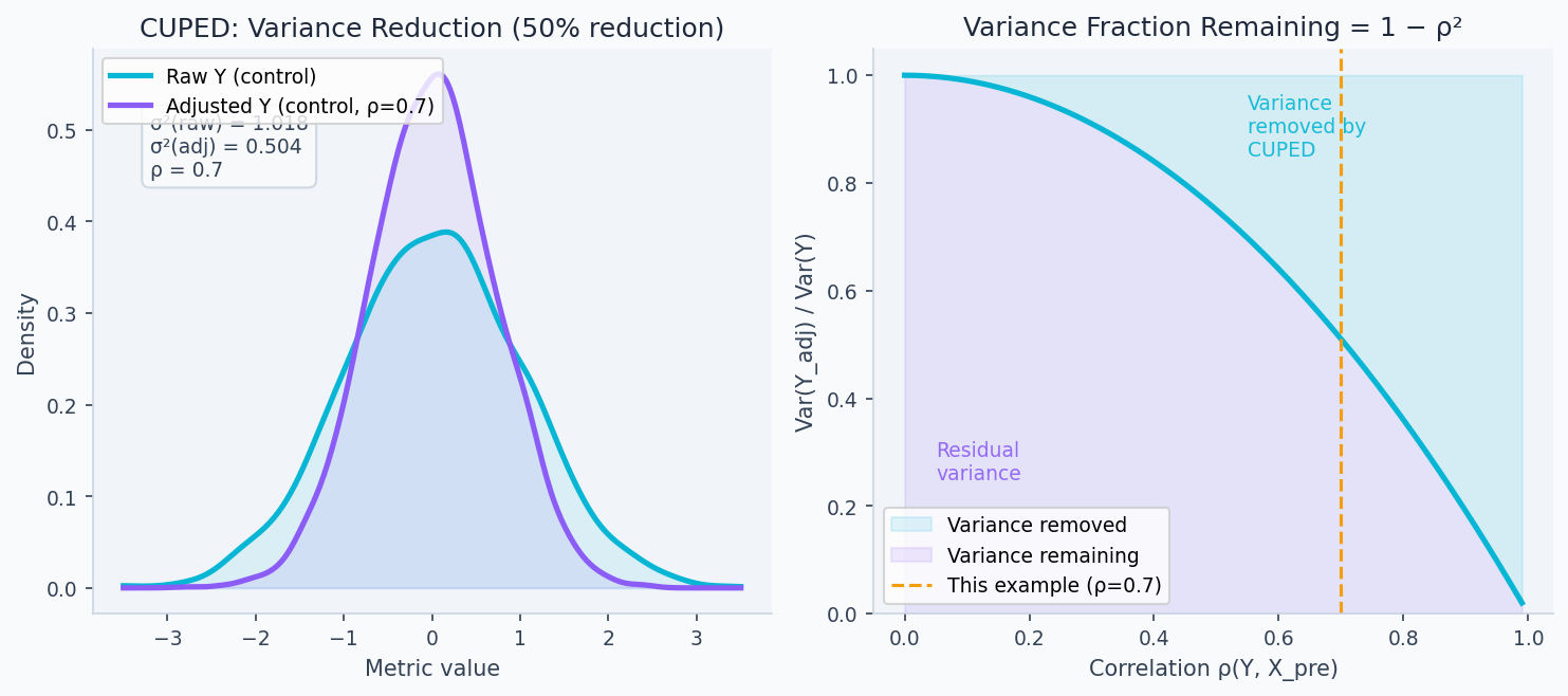
where $\rho = \text{Corr}(Y, X)$ . For Daily Active Users (DAU) with week-over-week stability $\rho = 0.8$ :

$\text{Var}(Y_{\text{adj}}) = \text{Var}(Y) \cdot (1 - 0.64) = 0.36 \cdot \text{Var}(Y)$

Same required number of standard errors, 64% less variance → 64% fewer users needed → 64% shorter experiment. The left panel below shows exactly this: the adjusted distribution is narrower, concentrating more probability mass near the true mean. The right panel shows that the variance remaining grows rapidly as $\rho$ falls — if your pre-experiment covariate has no predictive power, CUPED doesn't help.

$CUPED variance reduction: before vs after distributions, and variance fraction vs correlation$

Key properties:

Estimate $\hat{\theta}$ on the pooled dataset (both arms together), never per-arm — this avoids post-treatment contamination
The adjustment is unbiased regardless of $\hat{\theta}$ : $E[\hat{\tau}_{\text{adj}}] = \tau$ for any $\theta$ . Optimizing $\theta$ only minimizes variance.
Can be applied post-hoc at readout time if you forgot to pre-apply it

Ratio metrics and the delta method

Business metrics are often ratios: revenue per session = total revenue / total sessions. The naive variance formula $\text{Var}(X/Y) \approx \text{Var}(X)/\bar{Y}^2$ ignores the denominator's variability. The correct formula via the delta method:

$\text{Var}\!\left(\frac{\bar{X}}{\bar{Y}}\right) \approx \frac{1}{\bar{Y}^2}\left(\sigma_X^2 - 2\frac{\bar{X}}{\bar{Y}}\sigma_{XY} + \left(\frac{\bar{X}}{\bar{Y}}\right)^2 \sigma_Y^2\right)$

The covariance term $\sigma_{XY}$ matters. If sessions increase alongside revenue (treatment increases both numerator and denominator), the naive estimator will overstate variance. If sessions decrease while revenue increases, it will understate variance.

Design effect for cluster randomization

When SUTVA is violated — a treatment affecting one user spills over to others — you randomize at a higher level: cities, devices, households. The design effect (DEFF) quantifies the cost of cluster randomization versus individual randomization:

$\text{DEFF} = 1 + (m - 1) \cdot \rho_{\text{ICC}}$

where $m$ is average cluster size and $\rho_{\text{ICC}}$ is the intraclass correlation coefficient (ICC). For city-level experiments with $m = 50$ users/city and $\text{ICC} = 0.02$ :

$\text{DEFF} = 1 + 49 \times 0.02 = 1.98$

You need approximately twice as many users compared to user-level randomization. The effective sample size is $n_{\text{eff}} = n / \text{DEFF}$ . The ICC is often underestimated — cluster experiments are chronically underpowered as a result.

Stratified randomization

Rather than pure random assignment, stratified randomization assigns units within pre-specified strata (e.g., new vs. returning users, mobile vs. desktop). The variance reduction:

$\text{Var}(\hat{\tau}_{\text{stratified}}) = \text{Var}(\hat{\tau}_{\text{unstratified}}) - \frac{\sigma_{\text{between}}^2}{n}$

The reduction equals the between-stratum variance in outcomes divided by $n$ . For a metric where new vs. returning users differ significantly (large $\sigma_{\text{between}}^2$ ), stratification gives meaningful variance reduction with no statistical cost.

Walkthrough

CUPED implementation

python

import numpy as np
import pandas as pd
from scipy import stats
 
def apply_cuped(
    df: pd.DataFrame,
    outcome_col: str,
    pre_experiment_col: str,
    variant_col: str = 'variant',
) -> pd.Series:
    """
    CUPED-adjusted outcome.
    theta estimated on the full dataset (not per-arm) to avoid post-treatment bias.
    """
    X = df[pre_experiment_col].values
    Y = df[outcome_col].values
 
    # Estimate theta = Cov(Y, X) / Var(X) on pooled data
    theta = np.cov(Y, X)[0, 1] / np.var(X)
 
    # Adjust
    Y_adj = Y - theta * (X - X.mean())
    return pd.Series(Y_adj, index=df.index, name=f"{outcome_col}_cuped")
 
def variance_reduction_from_cuped(Y: np.ndarray, X: np.ndarray) -> dict:
    """How much variance does CUPED remove for this metric/covariate pair?"""
    rho = np.corrcoef(Y, X)[0, 1]
    return {
        "rho": round(rho, 3),
        "variance_reduction_pct": round((1 - rho**2) * 100, 1),
        "sample_size_reduction_pct": round((1 - rho**2) * 100, 1),  # same factor
    }
 
# Example: pre-experiment revenue as covariate for post-experiment revenue
df['revenue_cuped'] = apply_cuped(df, 'revenue_post', 'revenue_pre')
stats_pre = variance_reduction_from_cuped(df['revenue_post'].values, df['revenue_pre'].values)
# rho=0.72 → 48% variance reduction → 48% fewer users needed

Sample size with adjustments

python

import math
 
def sample_size_suite(
    baseline_rate: float,
    mde_relative: float,
    rho_cuped: float = 0.0,
    avg_cluster_size: float = 1.0,
    icc: float = 0.0,
    alpha: float = 0.05,
    power: float = 0.80,
) -> dict:
    """
    Sample size accounting for CUPED variance reduction and cluster design effect.
    """
    z_alpha = stats.norm.ppf(1 - alpha / 2)
    z_beta = stats.norm.ppf(power)
 
    delta = baseline_rate * mde_relative
    p_pool = baseline_rate + delta / 2
    sigma = math.sqrt(2 * p_pool * (1 - p_pool))
    n_base = math.ceil(((z_alpha + z_beta) * sigma / delta) ** 2)
 
    # Apply CUPED variance reduction
    n_cuped = math.ceil(n_base * (1 - rho_cuped**2))
 
    # Apply design effect for clustering
    deff = 1 + (avg_cluster_size - 1) * icc
    n_clustered = math.ceil(n_cuped * deff)
    n_clusters = math.ceil(n_clustered / avg_cluster_size) if avg_cluster_size > 1 else None
 
    return {
        "n_unadjusted": n_base,
        "n_with_cuped": n_cuped,
        "n_with_clustering": n_clustered,
        "n_clusters_needed": n_clusters,
        "design_effect": round(deff, 2),
        "days_needed": math.ceil(n_clustered / (200_000 * 0.5)),  # example traffic
    }
 
# Pure individual randomization: 45% baseline, 2% MDE
r = sample_size_suite(0.45, 0.02)
print(f"No adjustments: {r['n_unadjusted']:,} per arm")  # 19,652
 
# With CUPED (rho=0.7)
r = sample_size_suite(0.45, 0.02, rho_cuped=0.7)
print(f"With CUPED:     {r['n_with_cuped']:,} per arm")  # 10,718 (45% fewer)
 
# City-level randomization, 50 users/city, ICC=0.02
r = sample_size_suite(0.45, 0.02, avg_cluster_size=50, icc=0.02)
print(f"Cluster:        {r['n_clusters_needed']:,} clusters needed")  # 390

Ratio metric variance (delta method)

python

def ratio_metric_stats(
    numerator_A: np.ndarray,   # e.g., revenue per user in control
    denominator_A: np.ndarray, # e.g., sessions per user in control
    numerator_B: np.ndarray,
    denominator_B: np.ndarray,
) -> dict:
    """
    Compare ratio metrics (e.g., revenue per session) between arms.
    Uses delta method for variance of ratio.
    """
    def ratio_stats(num, den):
        r = num.mean() / den.mean()
        n = len(num)
        var_ratio = (1/den.mean()**2) * (
            np.var(num)
            - 2 * r * np.cov(num, den)[0,1]
            + r**2 * np.var(den)
        ) / n
        return r, var_ratio
 
    r_A, var_A = ratio_stats(numerator_A, denominator_A)
    r_B, var_B = ratio_stats(numerator_B, denominator_B)
 
    delta = r_B - r_A
    se = math.sqrt(var_A + var_B)
    z = delta / se
    p_value = 2 * (1 - stats.norm.cdf(abs(z)))
    ci = (delta - 1.96 * se, delta + 1.96 * se)
 
    return {
        "ratio_control": round(r_A, 4),
        "ratio_treatment": round(r_B, 4),
        "delta": round(delta, 4),
        "relative_lift_pct": round(delta / r_A * 100, 2),
        "ci_95": (round(ci[0], 4), round(ci[1], 4)),
        "p_value": round(p_value, 5),
    }

Randomization unit choice

The unit you randomize on determines what questions you can answer:

Unit	When to use	Tradeoffs
User ID	Most experiments — measures per-user effects	Cannot control SUTVA violations between users
Session ID	When user-level effects aren't relevant (e.g., anonymous search)	Same user may see both arms — "dilution"
Device ID	When the product is device-specific	Multi-device users dilute effects
City / Market	When SUTVA is violated (marketplace, social)	Cluster design effect reduces power significantly
Time period	Switchback experiments for marketplace pricing	Carry-over effects between periods

Always hash the randomization unit deterministically:

python

import hashlib
 
def assign_variant(unit_id: str, experiment_id: str, split: float = 0.5) -> str:
    """Deterministic, consistent assignment. Same user always gets same variant."""
    key = f"{experiment_id}:{unit_id}".encode()
    bucket = int(hashlib.sha256(key).hexdigest(), 16) % 10_000 / 10_000
    return "treatment" if bucket < split else "control"

Using a hash keyed on both experiment_id and unit_id ensures independence across experiments — the same user isn't always in the treatment arm.

Pre-experiment AA test

Simulate 1000 AA tests (no actual treatment) on historical data. Under a correctly specified variance model, exactly ~5% should yield p < 0.05. A higher false positive rate reveals a broken variance model.

python

def run_aa_simulation(
    user_metrics: np.ndarray,
    n_simulations: int = 1000,
    alpha: float = 0.05,
) -> dict:
    """
    Validate variance model by simulating AA tests on historical data.
    """
    false_positives = 0
    for _ in range(n_simulations):
        idx = np.random.permutation(len(user_metrics))
        mid = len(idx) // 2
        _, p = stats.ttest_ind(user_metrics[idx[:mid]], user_metrics[idx[mid:]])
        if p < alpha:
            false_positives += 1
 
    fpr = false_positives / n_simulations
    return {
        "false_positive_rate": round(fpr, 3),
        "expected": alpha,
        "verdict": "PASS" if abs(fpr - alpha) < 0.02 else "FAIL — check variance model",
        "likely_cause": (
            "clustering effects or autocorrelation" if fpr > alpha * 1.5 else "ok"
        ),
    }

Analysis & Evaluation

Where Your Intuition Breaks

Running a longer experiment always fixes an underpowered one. Sample size is determined by variance, not time. If your metric is dominated by high-variance users (e.g., a small fraction of users drive most revenue), doubling experiment duration barely helps — each new day adds the same noisy users. The fix is variance reduction (CUPED, winsorization, switching to a lower-CV metric), not more time. Duration matters only to the extent that it determines how many independent users you observe; for low-traffic products, even a month of runtime may fall short of the required n.

Metric selection: sensitivity vs. relevance

Not all metrics are equally useful as primary metrics. Two dimensions:

Sensitivity (statistical): how much signal per user. Measured by coefficient of variation ( $\text{CV} = \sigma / \mu$ ). Lower CV → smaller sample size for the same MDE.

Relevance (business): how predictive is this metric of long-term business outcomes? A metric can be easy to move (sensitive) but irrelevant (click-through on an interstitial you're about to remove).

The right primary metric maximizes both. Estimate relevance empirically: compute the correlation between candidate short-term metrics and long-term outcomes on historical data. Compute sensitivity using pre-experiment variance.

Metric	CV (lower is better)	Corr with 6-month retention
Sessions/week	0.8	0.71
Revenue/session	2.1	0.54
Search success rate	0.4	0.83 ← good primary
Feature adoption	0.6	0.31

Variance estimation from historical data

Use 4 weeks of pre-experiment data to estimate $\sigma^2$ . Apply a variance inflation factor of 1.1–1.2 to be conservative — this accounts for:

Users not yet in the experiment behaving differently from those who are
Week-of-month effects not captured in 4 weeks
Cross-device users counted once but generating multiple events

For highly right-skewed metrics (revenue, session duration), winsorize at the 99th percentile before estimating variance. The same winsorization threshold must be applied at analysis time.

Production-Ready Code

In production, CUPED runs as a post-processing step on the raw event data after experiment close — it doesn't require changing instrumentation. The key engineering decision is covariate selection: compute correlations on pre-experiment data and pick the highest-rho columns automatically. Assignment must use a deterministic hash so the same user always gets the same variant across sessions, devices, and service calls.

python

# production_experiment_design.py
# CUPED pipeline with automated covariate selection, sample size service,
# and deterministic variant assignment.
 
from __future__ import annotations
import hashlib, math
from typing import Sequence
import numpy as np
import pandas as pd
import scipy.stats as stats
 
 
# ── Covariate selection ───────────────────────────────────────────────────────
 
def select_cuped_covariates(
    df: pd.DataFrame,
    outcome_col: str,
    candidate_cols: Sequence[str],
    min_rho: float = 0.3,
) -> list[str]:
    """
    Returns pre-experiment columns with |rho| >= min_rho, sorted by descending |rho|.
    Only pass columns measured BEFORE experiment start as candidates.
    Typical candidates: last-week metric, last-month metric, days-since-signup.
    """
    Y = df[outcome_col].values
    ranked = []
    for col in candidate_cols:
        rho = float(np.corrcoef(Y, df[col].values)[0, 1])
        if abs(rho) >= min_rho:
            ranked.append((col, rho))
    ranked.sort(key=lambda x: abs(x[1]), reverse=True)
    return [col for col, _ in ranked]
 
 
# ── Multi-covariate CUPED via OLS residualisation ────────────────────────────
 
def apply_cuped_pipeline(
    df: pd.DataFrame,
    outcome_col: str,
    covariate_cols: Sequence[str],
    variant_col: str = "variant",
) -> pd.Series:
    """
    Generalises single-covariate CUPED to multiple covariates via OLS.
    theta is estimated on the POOLED dataset — never per arm — to avoid
    post-treatment contamination.
    Returns the adjusted outcome series indexed like df.
    """
    Y = df[outcome_col].values
    X = df[covariate_cols].values
    X_dm = X - X.mean(axis=0)                           # demean each covariate
    theta, *_ = np.linalg.lstsq(X_dm, Y, rcond=None)   # OLS minimises Var(Y_adj)
    Y_adj = Y - X_dm @ theta
    return pd.Series(Y_adj, index=df.index, name=f"{outcome_col}_cuped")
 
 
def cuped_variance_reduction(
    df: pd.DataFrame,
    outcome_col: str,
    covariate_cols: Sequence[str],
) -> dict:
    """How much variance does the covariate set explain? Use to justify covariate choice."""
    Y = df[outcome_col].values
    X = df[covariate_cols].values
    X_dm = X - X.mean(axis=0)
    theta, *_ = np.linalg.lstsq(X_dm, Y, rcond=None)
    Y_adj = Y - X_dm @ theta
    reduction = 1 - Y_adj.var() / Y.var()
    return {
        "covariates": list(covariate_cols),
        "variance_reduction_pct": round(reduction * 100, 1),
        "sample_size_reduction_pct": round(reduction * 100, 1),
    }
 
 
# ── Sample size service ───────────────────────────────────────────────────────
 
def sample_size_service(
    baseline: float,
    mde_relative: float,
    rho_cuped: float = 0.0,
    avg_cluster_size: float = 1.0,
    icc: float = 0.0,
    alpha: float = 0.05,
    power: float = 0.80,
) -> dict:
    """
    Single entry point for all experiment sizing. Accounts for CUPED variance
    reduction and cluster design effect in sequence.
    """
    z_a = stats.norm.ppf(1 - alpha / 2)
    z_b = stats.norm.ppf(power)
    delta = baseline * mde_relative
    p_pool = baseline + delta / 2
    sigma = math.sqrt(2 * p_pool * (1 - p_pool))
    n_base = math.ceil(((z_a + z_b) * sigma / delta) ** 2)
    n_cuped = math.ceil(n_base * (1 - rho_cuped ** 2))
    deff = 1 + (avg_cluster_size - 1) * icc
    n_final = math.ceil(n_cuped * deff)
    return {
        "n_per_arm_unadjusted": n_base,
        "n_per_arm_with_cuped": n_cuped,
        "n_per_arm_final": n_final,
        "n_clusters_needed": math.ceil(n_final / avg_cluster_size) if avg_cluster_size > 1 else None,
        "design_effect": round(deff, 3),
        "variance_reduction_pct": round(rho_cuped ** 2 * 100, 1),
    }
 
 
# ── Deterministic assignment ──────────────────────────────────────────────────
 
def assign_variant(
    unit_id: str,
    experiment_id: str,
    weights: dict[str, float] | None = None,
) -> str:
    """
    Deterministic assignment via SHA-256 bucket keyed on experiment+unit.
    Keying on both ensures the same user is not always in treatment across experiments.
    Supports multi-arm splits via a weights dict that must sum to 1.0.
    """
    weights = weights or {"control": 0.5, "treatment": 0.5}
    assert abs(sum(weights.values()) - 1.0) < 1e-9, "Weights must sum to 1"
    key = f"{experiment_id}:{unit_id}".encode()
    bucket = int(hashlib.sha256(key).hexdigest(), 16) % 1_000_000 / 1_000_000
    cumulative = 0.0
    for arm, w in weights.items():
        cumulative += w
        if bucket < cumulative:
            return arm
    return list(weights)[-1]   # floating-point safety valve
 
 
# ── Example ───────────────────────────────────────────────────────────────────
print(sample_size_service(0.45, 0.02, rho_cuped=0.72))
# {'n_per_arm_unadjusted': 19652, 'n_per_arm_with_cuped': 10991, ...}
 
print(assign_variant("user_8675309", "checkout_v2_2026q2"))   # same every time
print(assign_variant("user_8675309", "onboarding_v3_2026q2")) # different experiment

Enjoying these notes?

Get new lessons delivered to your inbox. No spam.

Hypothesis Testing

Validity Threats