Hypothesis Testing

Every time a tech company ships a feature — a new recommendation algorithm, a checkout flow change, an onboarding tweak — they're making a decision with incomplete information. The question isn't "did the metric go up?" It's "would the metric have gone up anyway?" Statistical hypothesis testing is the machinery that separates real signal from noise in randomized experiments. A product team that doesn't understand statistical power will run underpowered experiments and miss real effects, shipping nothing when something exists. A team that misreads p-values will ship features that don't actually work. The core framework has three interlocking pieces: framing what error you're willing to tolerate, computing the test statistic, and deciding what the result means — which requires understanding the gap between statistical significance and practical significance.

Theory

A/B Test — Sampling Distributions of the Mean

Effect size (δ)0.50σ

Sample size (n/arm)200

α =

z = 5.00p = <0.001power = 100%SIGNIFICANT

Power vs sample size — effect size δ = 0.50σ, α = 0.05

Amber dot = current n. Green dashed = 80% power target (industry standard). Power ∝ √n × δ.

Control (A)

Treatment (B)

Critical threshold

Every A/B test is answering one question: did the treatment cause the difference, or would you have seen it anyway in two groups of identical users? The distribution of possible outcomes under no effect is what the null hypothesis describes — if the observed difference falls far in the tail of that distribution, you have grounds to reject it. The diagram above shows the two overlapping sampling distributions: when they barely separate (small effect, small n), no test can tell them apart.

The hypothesis testing framework

An A/B test is a randomized controlled experiment. You split users into two groups at random, expose one to a change (treatment), leave the other unchanged (control), then test whether the observed difference in outcomes is real or just noise.

The formal framework (Neyman-Pearson):

Null hypothesis $H_0$ : the treatment has no effect, $\mu_B = \mu_A$
Alternative hypothesis $H_1$ : the treatment has an effect, $\mu_B \neq \mu_A$

You never prove $H_0$ false. You compute the probability of seeing your data (or more extreme) if $H_0$ were true. If that probability is low enough, you reject $H_0$ .

Type I and Type II errors

	$H_0$ true (no effect)	$H_0$ false (effect exists)
Reject $H_0$	Type I error (false positive, rate $\alpha$ )	Correct (true positive, rate $1-\beta$ )
Fail to reject $H_0$	Correct (true negative, rate $1-\alpha$ )	Type II error (false negative, rate $\beta$ )

Standard choices: $\alpha = 0.05$ (5% false positive rate) and $\beta = 0.20$ (80% power). These are not universal laws — they're business decisions. For safety-critical features, use $\alpha = 0.01$ . For high-velocity product iteration with many experiments, $\alpha = 0.05$ is common but power 0.90 is safer.

The tradeoff: lowering $\alpha$ reduces false positives but increases false negatives (requires larger $n$ ). Increasing power requires larger $n$ or lower $\alpha$ .

The test statistic

For comparing two means (continuous metric), the two-sample Z-test (or Welch's t-test for small samples):

$Z = \frac{\bar{X}_B - \bar{X}_A}{\sqrt{\frac{\sigma_A^2}{n_A} + \frac{\sigma_B^2}{n_B}}}$

The denominator $\sqrt{\sigma_A^2/n_A + \sigma_B^2/n_B}$ is the standard error of the difference — the only scale that makes the numerator interpretable. Without dividing by it, a difference of 0.01 on a metric with $\sigma = 0.001$ would look identical to the same difference on a metric with $\sigma = 10$ , even though the first is a massive signal and the second is indistinguishable from noise. The Z-statistic is meaningful precisely because it expresses the observed difference in units of how variable that difference would be under random assignment.

Under $H_0$ , $Z \sim \mathcal{N}(0, 1)$ for large $n$ . Reject $H_0$ when $|Z| > z_{\alpha/2} = 1.96$ for $\alpha = 0.05$ .

For a proportion metric (binary outcome like conversion), use:

$Z = \frac{\hat{p}_B - \hat{p}_A}{\sqrt{\hat{p}(1-\hat{p})\left(\frac{1}{n_A} + \frac{1}{n_B}\right)}}$

where $\hat{p} = (n_A \hat{p}_A + n_B \hat{p}_B)/(n_A + n_B)$ is the pooled proportion under $H_0$ .

The p-value

The p-value is the probability of observing a test statistic at least as extreme as the one computed, assuming $H_0$ is true:

$p = P(|Z| \geq |z_{\text{obs}}| \mid H_0)$

What a p-value is not:

It is not the probability that $H_0$ is true
It is not the probability that the result occurred by chance
It is not the size of the effect

A p-value of 0.03 means: if there were truly no effect, you'd see a difference this large or larger only 3% of the time. It says nothing about whether the effect is practically meaningful.

Minimum Detectable Effect (MDE)

The MDE is the smallest true effect you can detect with probability $1 - \beta$ at significance level $\alpha$ :

$\text{MDE} = (z_{\alpha/2} + z_\beta) \cdot \sqrt{\frac{\sigma_A^2}{n_A} + \frac{\sigma_B^2}{n_B}}$

For equal arms ( $n_A = n_B = n$ ) and equal variance $\sigma^2$ :

$\text{MDE} = (z_{\alpha/2} + z_\beta) \cdot \sigma\sqrt{\frac{2}{n}}$

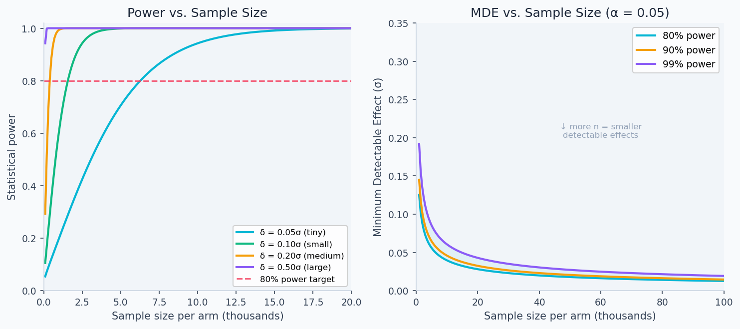
For $n = 10{,}000$ , $\sigma = 1$ , $\alpha = 0.05$ , $\beta = 0.20$ : $\text{MDE} = 2.80 \cdot \sqrt{2/10{,}000} \approx 0.040\sigma$ . Doubling $n$ to 20,000 reduces MDE by $1/\sqrt{2} \approx 29\%$ .

Power curve

Power as a function of true effect $\delta$ , sample size $n$ , variance $\sigma^2$ :

$\text{Power}(\delta, n) = \Phi\!\left(\frac{|\delta|}{\sigma}\sqrt{\frac{n}{2}} - z_{\alpha/2}\right)$

Monotonically increasing in $|\delta|$ and $n$ , decreasing in $\sigma$ and $\alpha$ .

The left panel shows that detecting a 5% relative lift on a metric with high variance requires orders of magnitude more users than detecting a 50% lift. The right panel shows the MDE as a function of sample size — investing in more traffic directly shrinks the smallest effect you can reliably detect.

Confidence intervals

A confidence interval gives the range of effect sizes consistent with your data. For a 95% CI:

$\hat{\delta} \pm z_{0.025} \cdot \hat{\sigma}_\delta = \hat{\delta} \pm 1.96 \cdot \sqrt{\frac{\hat{\sigma}_A^2}{n_A} + \frac{\hat{\sigma}_B^2}{n_B}}$

The CI is more informative than the p-value alone. An experiment with $p = 0.001$ and CI = [+0.01%, +0.5%] signals a real but tiny effect. An experiment with $p = 0.08$ and CI = [-0.1%, +3.2%] signals a potentially large effect but an underpowered experiment. The width is what matters.

Walkthrough

End-to-end test of a conversion rate

python

import numpy as np
from scipy import stats
import math
 
def ab_test_proportions(
    n_control: int,
    n_treatment: int,
    conversions_control: int,
    conversions_treatment: int,
    alpha: float = 0.05,
) -> dict:
    """
    Two-sided Z-test for a binary conversion metric.
    Uses pooled proportion under H0.
    """
    p_c = conversions_control / n_control
    p_t = conversions_treatment / n_treatment
    p_pool = (conversions_control + conversions_treatment) / (n_control + n_treatment)
 
    # Test statistic
    se_pool = math.sqrt(p_pool * (1 - p_pool) * (1/n_control + 1/n_treatment))
    z = (p_t - p_c) / se_pool
    p_value = 2 * (1 - stats.norm.cdf(abs(z)))
 
    # Confidence interval (unpooled SE)
    se_unpooled = math.sqrt(p_c*(1-p_c)/n_control + p_t*(1-p_t)/n_treatment)
    delta = p_t - p_c
    ci = (delta - 1.96 * se_unpooled, delta + 1.96 * se_unpooled)
    ci_relative = (ci[0]/p_c * 100, ci[1]/p_c * 100)
 
    return {
        "conversion_control": round(p_c, 4),
        "conversion_treatment": round(p_t, 4),
        "relative_lift_pct": round(delta / p_c * 100, 2),
        "ci_95_relative": (round(ci_relative[0], 2), round(ci_relative[1], 2)),
        "z_stat": round(z, 4),
        "p_value": round(p_value, 5),
        "significant": p_value < alpha,
    }
 
# Example: 45% baseline, treatment shows 46.3%
result = ab_test_proportions(
    n_control=20_000, n_treatment=20_000,
    conversions_control=9_000, conversions_treatment=9_260,
)
# relative_lift: +2.9%, CI: [+1.1%, +4.6%], p=0.0018 → significant

Sample size calculation

python

def required_sample_size(
    baseline_rate: float,
    mde_relative: float,
    alpha: float = 0.05,
    power: float = 0.80,
) -> int:
    """Sample size per arm for a proportion metric."""
    delta = baseline_rate * mde_relative
    p2 = baseline_rate + delta
    p_pool = (baseline_rate + p2) / 2
    sigma = math.sqrt(2 * p_pool * (1 - p_pool))
    z_alpha = stats.norm.ppf(1 - alpha / 2)
    z_beta = stats.norm.ppf(power)
    n = ((z_alpha + z_beta) * sigma / delta) ** 2
    return math.ceil(n)
 
def required_sample_size_continuous(
    std: float,
    mde_absolute: float,
    alpha: float = 0.05,
    power: float = 0.80,
) -> int:
    """Sample size per arm for a continuous metric."""
    z_alpha = stats.norm.ppf(1 - alpha / 2)
    z_beta = stats.norm.ppf(power)
    n = 2 * ((z_alpha + z_beta) * std / mde_absolute) ** 2
    return math.ceil(n)
 
# 45% baseline conversion, detect 2% relative lift (0.9 pp)
n = required_sample_size(0.45, 0.02)
print(f"{n:,} users per arm")  # → 19,652
 
# Revenue: mean=$2.50, std=$8, detect $0.10 lift
n = required_sample_size_continuous(std=8, mde_absolute=0.10)
print(f"{n:,} users per arm")  # → 49,281

Pre-registering your analysis

Write down your primary metric, MDE, $\alpha$ , power, and analysis plan before the experiment starts. Store it in the experiment doc:

Primary metric: conversion_rate
MDE: 2% relative lift (absolute: 0.009)
Alpha: 0.05 (two-sided)
Power: 0.80
Sample size: 19,652 per arm
Duration: 14 days (based on 2,800 eligible users/day)

Analysis: two-sided Z-test on proportions, winsorize revenue at p99
Decision rule: ship if p < 0.05 AND CI lower bound > 1% relative

Pre-registration prevents Hypothesizing After Results are Known (HARKing): adjusting your hypothesis after seeing the data to match whatever moved. It's the single highest-leverage practice in experiment credibility.

🚀Production

Mature experimentation platforms require researchers to lock down the primary metric and statistical test before the experiment launches. The analysis plan is immutable — you can add secondary metrics to explore, but the primary decision is pre-committed. Teams that skip this regularly "discover" significant results by shopping across 15 metrics until one crosses p=0.05.

Practical vs. statistical significance

The 2×2 decision matrix:

python

def interpret_result(
    p_value: float,
    ci_lower: float,      # lower bound of 95% CI on relative lift
    ci_upper: float,      # upper bound of 95% CI on relative lift
    mde: float,           # minimum practically significant lift (e.g., 0.02 for 2%)
    alpha: float = 0.05,
) -> str:
    stat_sig = p_value < alpha
    prac_sig_lower = ci_lower > mde  # CI lower bound above MDE → clearly practical
 
    if stat_sig and prac_sig_lower:
        return "SHIP: statistically and practically significant"
    if stat_sig and not prac_sig_lower:
        return "NULL RESULT: significant but below MDE — effect too small to matter"
    if not stat_sig and ci_upper > mde:
        return "UNDERPOWERED: effect could be real and large — extend experiment"
    return "NO EFFECT: fully powered null result"

Analysis & Evaluation

Where Your Intuition Breaks

A statistically significant result means the treatment worked. Statistical significance means the effect is unlikely to be zero — not that it is large enough to matter. A 0.01% lift on conversion rate can be statistically significant at n=1,000,000 but is economically meaningless. The confidence interval lower bound tells you whether the effect is practically significant: a CI of [+0.001%, +0.02%] is a null result even if p=0.001. Always interpret effect size and confidence interval bounds, not just the p-value.

Bayesian interpretation for underpowered experiments

When a frequentist test says "not significant," a Bayesian update gives the posterior probability that the effect exceeds a threshold. This is especially useful for short experiments or when you ran with less traffic than planned.

python

def bayesian_update(
    delta_hat: float,       # observed effect estimate
    se_delta: float,        # standard error of estimate
    prior_mean: float = 0.0,
    prior_std: float = 0.03,  # prior uncertainty (set to expected effect range)
    mde: float = 0.01,
) -> dict:
    """Gaussian conjugate posterior for experiment effect."""
    prior_prec = 1 / prior_std**2
    like_prec = 1 / se_delta**2
    post_prec = prior_prec + like_prec
 
    post_mean = (prior_mean * prior_prec + delta_hat * like_prec) / post_prec
    post_std = math.sqrt(1 / post_prec)
 
    prob_positive = 1 - stats.norm.cdf(0, post_mean, post_std)
    prob_above_mde = 1 - stats.norm.cdf(mde, post_mean, post_std)
 
    return {
        "posterior_mean": round(post_mean, 5),
        "prob_effect_positive": round(prob_positive, 3),
        "prob_above_mde": round(prob_above_mde, 3),
        "credible_interval_95": tuple(
            round(x, 5) for x in stats.norm.interval(0.95, post_mean, post_std)
        ),
    }

Common misinterpretations

Claim	Wrong	Right
"p = 0.04, so there's a 4% chance the result is due to chance"	✗	p-value conditions on $H_0$ being true; it doesn't give $P(H_0)$
"p > 0.05 means no effect"	✗	Fail to reject — the effect may exist but be undetected (low power)
"We replicated, so the effect is confirmed"	✗	Two p < 0.05 results still have ~10% joint false positive rate
"The CI [+0.1%, +3.5%] shows the true effect"	✗	95% of CIs from this procedure will contain the true effect — not this specific one

Production-Ready Code

A production experiment platform centralises three things: the experiment config (pre-registered before launch), the readout logic (called once at the pre-registered sample size), and the alerting pipeline. Pre-registration is the single most impactful practice — locking the primary metric, $\alpha$ , power, and MDE before launch prevents HARKing and makes the decision rule auditable.

python

# experiment_platform.py
# Statsig-style experiment schema, automated readout, and significance alerting.
 
from dataclasses import dataclass
import math, json
import numpy as np
import scipy.stats as stats
 
 
@dataclass
class ExperimentConfig:
    experiment_id: str
    primary_metric: str
    mde_relative: float      # e.g. 0.02 for 2%
    baseline: float          # historical metric value (proportion or mean)
    alpha: float = 0.05
    power: float = 0.80
    two_sided: bool = True
 
 
def precompute_sample_size(cfg: ExperimentConfig) -> int:
    """
    Lock in required n before launch — baked into the experiment record.
    Stored in the experiment DB so readout logic can assert the experiment
    ran to completion before declaring results.
    """
    delta = cfg.baseline * cfg.mde_relative
    p_pool = cfg.baseline + delta / 2
    sigma = math.sqrt(2 * p_pool * (1 - p_pool))
    z_alpha = stats.norm.ppf(1 - cfg.alpha / 2 if cfg.two_sided else 1 - cfg.alpha)
    z_beta = stats.norm.ppf(cfg.power)
    return math.ceil(((z_alpha + z_beta) * sigma / delta) ** 2)
 
 
def readout(
    cfg: ExperimentConfig,
    control: np.ndarray,
    treatment: np.ndarray,
) -> dict:
    """
    Automated readout. Call once experiment reaches pre-registered sample size.
    Returns a structured result dict consumed by the decision layer and dashboards.
    """
    n_c, n_t = len(control), len(treatment)
    mean_c, mean_t = control.mean(), treatment.mean()
    se = math.sqrt(control.var() / n_c + treatment.var() / n_t)
    delta = mean_t - mean_c
    z = delta / se
    p = 2 * (1 - stats.norm.cdf(abs(z))) if cfg.two_sided else 1 - stats.norm.cdf(z)
    ci = (delta - 1.96 * se, delta + 1.96 * se)
    required_n = precompute_sample_size(cfg)
    mde_abs = cfg.baseline * cfg.mde_relative
 
    stat_sig = p < cfg.alpha
    prac_sig = ci[0] > mde_abs
 
    if stat_sig and prac_sig:
        decision = "SHIP"
    elif stat_sig and not prac_sig:
        decision = "NULL — significant but below MDE"
    elif not stat_sig and ci[1] > mde_abs:
        decision = "EXTEND — underpowered, effect could be real and large"
    else:
        decision = "NO EFFECT — fully powered null result"
 
    return {
        "experiment_id": cfg.experiment_id,
        "status": "complete" if min(n_c, n_t) >= required_n else "underpowered",
        "n_control": n_c,
        "n_treatment": n_t,
        "required_n_per_arm": required_n,
        "delta": round(delta, 6),
        "relative_lift_pct": round(delta / mean_c * 100, 3),
        "ci_95": (round(ci[0], 6), round(ci[1], 6)),
        "p_value": round(p, 6),
        "significant": stat_sig,
        "decision": decision,
    }
 
 
def alert_on_significance(result: dict, webhook_url: str | None = None) -> None:
    """
    Post a structured alert when an experiment reaches significance.
    Replace print() with your alerting backend (Slack webhook, PagerDuty, etc.).
    Only alert on SHIP decisions — avoid noisy alerts for underpowered or null results.
    """
    if result["decision"] == "SHIP":
        payload = {
            "experiment_id": result["experiment_id"],
            "decision": result["decision"],
            "relative_lift_pct": result["relative_lift_pct"],
            "p_value": result["p_value"],
            "ci_95": result["ci_95"],
        }
        if webhook_url:
            import urllib.request
            req = urllib.request.Request(
                webhook_url,
                data=json.dumps(payload).encode(),
                headers={"Content-Type": "application/json"},
                method="POST",
            )
            urllib.request.urlopen(req)
        else:
            print(f"[EXPERIMENT ALERT] {json.dumps(payload, indent=2)}")
 
 
# ── Example ───────────────────────────────────────────────────────────────────
cfg = ExperimentConfig(
    experiment_id="checkout_v2_2026q2",
    primary_metric="conversion_rate",
    mde_relative=0.02,
    baseline=0.45,
)
required_n = precompute_sample_size(cfg)
print(f"Required n per arm: {required_n:,}")  # 19,652
 
rng = np.random.default_rng(42)
control   = rng.binomial(1, 0.450, required_n).astype(float)
treatment = rng.binomial(1, 0.459, required_n).astype(float)  # true +2% lift
result = readout(cfg, control, treatment)
print(json.dumps(result, indent=2))
alert_on_significance(result)

Enjoying these notes?

Get new lessons delivered to your inbox. No spam.

Specialized

Reinforcement Learning Fundamentals

Experimental Design