Requires:Experimental Design

Validity Threats

A well-designed experiment with a correctly pre-registered analysis plan can still fail — not because the statistics are wrong, but because the experimental machinery breaks down in practice. The most persistent sources of failure are behavioral: checking results daily and stopping when you see $p < 0.05$ (peeking), running experiments where the two arms received different numbers of users despite a 50/50 split (SRM), and declaring significance on whichever of 15 secondary metrics crossed a threshold first (multiple testing). Each of these has a rigorous fix. Sequential testing lets you monitor continuously without inflating error rates. SRM detection catches logging bugs before you trust the results. Benjamini-Hochberg controls the false discovery rate across a portfolio of metrics. Understanding these threats is what separates an experiment platform that produces trustworthy signals from one that produces optimistic noise.

Theory

Sequential Testing

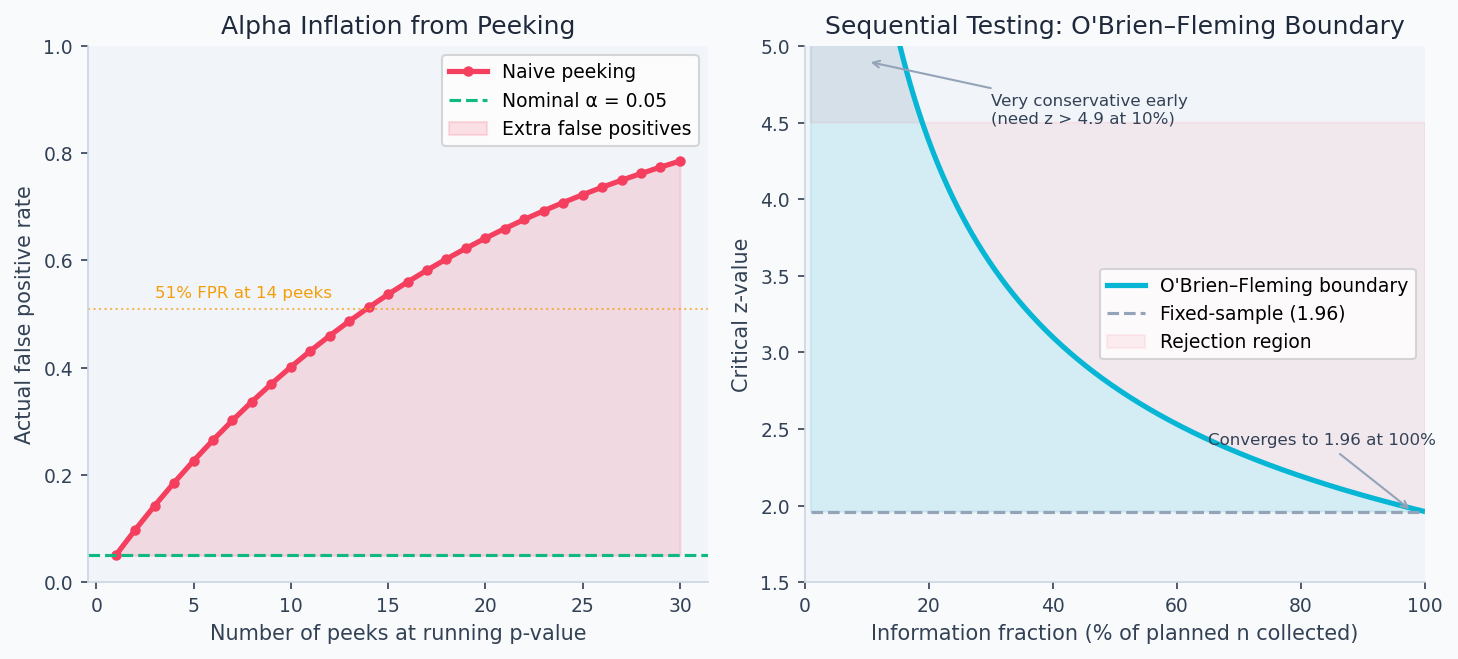
Peeking at the fixed threshold inflates Type I error — the Z-statistic crosses 1.96 by chance mid-experiment. The O'Brien-Fleming boundary is higher early (conservative) and converges to 1.96 only at the final look.

Checking a live experiment's p-value every day feels harmless, but it multiplies your false positive rate the same way running 14 independent tests would. The Z-statistic is a random walk under the null — given enough time, it will cross 1.96 by chance even when no effect exists. Sequential testing methods work by pre-budgeting how much false positive risk you spend at each peek, so the total across all planned checks still equals your target α.

The peeking problem

The most common experiment mistake is stopping when you see $p < 0.05$ before the planned end date. This inflates your false positive rate dramatically.

Under repeated testing at $\alpha = 0.05$ with a fixed $n$ , if you peek every day for $k$ days and stop when significant, your true false positive rate grows approximately as:

$\alpha_{\text{actual}} \approx 1 - (1 - \alpha)^k$

This formula treats each peek as independent, which slightly overstates inflation (peeks on the same growing dataset are correlated), but the qualitative conclusion is correct: each additional look consumes part of your error budget. Sequential testing methods like O'Brien-Fleming solve this by setting each peek's threshold high enough that the cumulative alpha spending across all planned peeks exactly equals the pre-specified $\alpha$ — the budget is fixed; only how it is spent across time changes.

For 14 daily peeks: $\alpha_{\text{actual}} \approx 1 - 0.95^{14} \approx 0.51$ . You'd call 51% of null experiments "significant." This is not a theoretical concern — it is the most reliably reproduced error in A/B testing practice.

The root cause is that the Z-statistic follows a random walk under $H_0$ . If you wait long enough, it will eventually cross 1.96 by chance even when there is no effect. Fixing $n$ in advance and analyzing once is the classical remedy. But business pressure to ship fast makes continuous monitoring irresistible.

Sequential testing

Sequential testing provides valid inference at any stopping time. The mixture Sequential Probability Ratio Test (mSPRT) constructs a test martingale $M_t$ that satisfies $E[M_t | H_0] \leq 1$ at all $t$ . By Ville's inequality:

$P\!\left(\exists t: M_t \geq 1/\alpha\right) \leq \alpha$

You can stop and declare significance as soon as $M_t \geq 1/\alpha$ , with guaranteed type-I error $\leq \alpha$ . This is always-valid: you can peek as often as you want.

In practice, the Lan-DeMets alpha spending approach is simpler and more widely used. It plans $k$ interim analyses and "spends" the $\alpha$ budget across them. The O'Brien-Fleming spending function is very conservative early (requiring a large effect to stop at the first interim) and nearly standard at the final analysis:

$\alpha_{\text{spent}}(t) = 2 - 2\Phi\!\left(\frac{z_{\alpha/2}}{\sqrt{t/T}}\right)$

where $t$ is current information fraction ( $n_t / N$ ). The critical z-value at information fraction $t$ is $z_t = z_{\alpha/2}/\sqrt{t/T}$ .

The cost: sequential tests require 5–30% more expected sample size under $H_1$ compared to a fixed-sample test. The gain is the ability to stop early when effects are large.

The left panel below shows how rapidly naive peeking inflates the false positive rate — 14 peeks at $\alpha = 0.05$ pushes the actual FPR to 51%. The right panel shows the O'Brien-Fleming boundary: the critical z-value required for significance starts very high (protecting against early false positives) and converges toward 1.96 only at the planned end date.

Alpha inflation from peeking and O'Brien-Fleming sequential boundary

Sample Ratio Mismatch (SRM)

An SRM occurs when the observed assignment ratio differs significantly from expected. For a planned 50/50 split:

$X^2 = \frac{(O_A - E_A)^2}{E_A} + \frac{(O_B - E_B)^2}{E_B} \sim \chi^2(1)$

where $E_A = E_B = (O_A + O_B)/2$ . Standard threshold: $p < 0.001$ .

An SRM is not a statistical nuisance — it means the two arms are not comparable populations. Any treatment effect estimate from an SRM experiment is invalid. The most common cause is not imbalanced randomization, but a logging bug that fires events in one arm but not the other.

Multiple testing (FWER and FDR)

When testing $K$ metrics simultaneously, the probability of at least one false positive — the Family-Wise Error Rate (FWER) — is:

$\text{FWER} = 1 - (1 - \alpha)^K$

For $K = 10$ at $\alpha = 0.05$ : $\text{FWER} \approx 0.40$ . You expect 4 spurious "discoveries" in every 10-metric readout.

Bonferroni correction: reject $H_{0,k}$ if $p_k < \alpha/K$ . Controls FWER at $\alpha$ but is conservative.

The False Discovery Rate (FDR) is less restrictive: it controls the expected proportion of rejections that are false positives. The Benjamini-Hochberg (BH) procedure:

Sort p-values: $p_{(1)} \leq p_{(2)} \leq \cdots \leq p_{(K)}$
Find the largest $k$ such that $p_{(k)} \leq \frac{k}{K} \cdot q$
Reject all $H_{0,(i)}$ for $i \leq k$

BH controls FDR at $q$ and is more powerful than Bonferroni. For $K = 10$ , $q = 0.05$ : BH rejects more true effects than Bonferroni.

SUTVA and network effects

SUTVA (Stable Unit Treatment Value Assumption) requires that unit $i$ 's outcome depends only on $i$ 's treatment, not on others'. Violations arise in:

Social networks: treating user A changes content user B sees
Marketplaces: a pricing treatment on sellers affects buyers
Shared infrastructure: treatment arm uses more compute, degrading control latency

When SUTVA is violated, the naive ATE estimator is biased. The treatment effect measured in a user-level A/B test includes the direct effect on treated users plus spillover effects on their neighbors, but not the platform-wide equilibrium effect of treating everyone.

Total Average Treatment Effect (TATE) vs. Direct Average Treatment Effect (DATE): $\tau_{\text{TATE}} = E[Y_i(\mathbf{1}) - Y_i(\mathbf{0})] \neq E[Y_i(1, \mathbf{T}_{-i}) - Y_i(0, \mathbf{T}_{-i})]$

where $\mathbf{1}$ is the vector of all-treatment and $\mathbf{T}_{-i}$ is neighbors' treatment assignment.

Walkthrough

Sequential test with alpha spending

python

import numpy as np
from scipy import stats
import math
 
def obrien_fleming_boundary(
    info_fraction: float,  # t/T, fraction of planned sample collected so far
    alpha: float = 0.05,
) -> float:
    """
    Critical z-value at given information fraction under O'Brien-Fleming spending.
    Very conservative early (large z required), relaxes toward 1.96 at t=T.
    """
    alpha_spent = 2 * (1 - stats.norm.cdf(
        stats.norm.ppf(1 - alpha / 2) / math.sqrt(info_fraction)
    ))
    return stats.norm.ppf(1 - alpha_spent / 2)
 
def sequential_test(
    observations_A: list,   # growing list of outcomes for control
    observations_B: list,   # growing list of outcomes for treatment
    n_planned: int,          # planned final sample size per arm
    alpha: float = 0.05,
) -> dict:
    """
    Run sequential test at current information fraction.
    Safe to call at any time without alpha inflation.
    """
    n = min(len(observations_A), len(observations_B))
    info_fraction = min(n / n_planned, 1.0)
    z_boundary = obrien_fleming_boundary(info_fraction, alpha)
 
    A = np.array(observations_A[:n])
    B = np.array(observations_B[:n])
    delta = B.mean() - A.mean()
    se = math.sqrt(A.var()/n + B.var()/n)
    z_obs = delta / se if se > 0 else 0
 
    return {
        "n_per_arm": n,
        "info_fraction": round(info_fraction, 3),
        "z_observed": round(z_obs, 4),
        "z_boundary": round(z_boundary, 4),
        "can_stop_significant": abs(z_obs) > z_boundary,
        "delta": round(delta, 5),
        "p_value": round(2 * (1 - stats.norm.cdf(abs(z_obs))), 5),
    }
 
# Check at 25%, 50%, 75%, 100% of planned n=20,000
T = 20_000
for pct in [0.25, 0.50, 0.75, 1.00]:
    z = obrien_fleming_boundary(pct)
    print(f"t={pct:.0%}: z_boundary={z:.3f}  (fixed-sample: 1.960)")
# t=25%: z_boundary=2.797  ← need large z to stop early
# t=50%: z_boundary=2.306
# t=75%: z_boundary=2.094
# t=100%: z_boundary=1.971  ← nearly the same as fixed-sample

SRM detection

python

from scipy.stats import chi2
 
def check_srm(
    n_control: int,
    n_treatment: int,
    expected_split: float = 0.5,
    threshold: float = 0.001,
) -> dict:
    """Chi-square test for Sample Ratio Mismatch."""
    n_total = n_control + n_treatment
    E_c = n_total * (1 - expected_split)
    E_t = n_total * expected_split
 
    chi2_stat = (n_control - E_c)**2/E_c + (n_treatment - E_t)**2/E_t
    p_value = 1 - chi2.cdf(chi2_stat, df=1)
 
    return {
        "observed_split": round(n_treatment / n_total, 4),
        "expected_split": expected_split,
        "chi2": round(chi2_stat, 4),
        "p_value": round(p_value, 6),
        "srm_detected": p_value < threshold,
        "action": "STOP — do not interpret results" if p_value < threshold else "OK",
    }

Common SRM causes and fixes:

Root cause	Signature	Fix
Logging bug (one arm only)	Ratio is exactly 50:50 in event count but not user count	Fix logging; restart
Bot filtering only in treatment	Treatment has fewer users	Apply bot filter before bucketing
Client-side bucketing with caching	Users re-bucketed on return visit	Move bucketing server-side
Hash collision in assignment	Predictable bucketing pattern	Use SHA-256 keyed on experiment ID
Cache hit asymmetry	Latency metric is biased even in AA	Add cache warming to both arms

Multiple testing correction

python

import numpy as np
 
def benjamini_hochberg(p_values: list, q: float = 0.05) -> list:
    """
    Benjamini-Hochberg procedure for FDR control.
    Returns a list of booleans: True = reject H0 for that metric.
    """
    K = len(p_values)
    sorted_idx = np.argsort(p_values)
    sorted_p = np.array(p_values)[sorted_idx]
 
    # BH threshold: p(k) <= k/K * q
    thresholds = np.arange(1, K+1) / K * q
    below = sorted_p <= thresholds
 
    # Find largest k where condition holds, reject all k' <= k
    if not below.any():
        reject_sorted = np.zeros(K, dtype=bool)
    else:
        k_star = np.where(below)[0].max()
        reject_sorted = np.arange(K) <= k_star
 
    reject = np.zeros(K, dtype=bool)
    reject[sorted_idx] = reject_sorted
 
    return reject.tolist()
 
# Example: 10 secondary metrics
metrics = ['CTR', 'add_to_cart', 'session_len', 'zero_results', 'bounce_rate',
           'pages_per_session', 'return_rate', 'share_rate', 'scroll_depth', 'search_count']
p_values = [0.001, 0.045, 0.11, 0.032, 0.28, 0.73, 0.041, 0.22, 0.68, 0.009]
 
rejections = benjamini_hochberg(p_values, q=0.05)
for metric, p, reject in zip(metrics, p_values, rejections):
    print(f"{metric}: p={p:.3f}  {'✅ reject' if reject else '— retain'}")

Switchback experiments for SUTVA violations

When user-level randomization violates SUTVA (marketplace pricing, social features), randomize at the time period level instead. Alternate between treatment and control on a fixed schedule (e.g., 30-minute windows):

python

import hashlib
import datetime
 
def get_switchback_assignment(
    timestamp: datetime.datetime,
    experiment_id: str,
    window_minutes: int = 30,
) -> str:
    """
    Returns 'treatment' or 'control' based on which time window the timestamp falls in.
    Deterministic: same timestamp always gets same assignment.
    """
    window_index = int(timestamp.timestamp() // (window_minutes * 60))
    key = f"{experiment_id}:{window_index}".encode()
    bucket = int(hashlib.sha256(key).hexdigest(), 16) % 2
    return "treatment" if bucket == 0 else "control"

The identifying assumption: no carry-over between periods (outcomes in period $t$ don't depend on treatment in period $t-1$ ). For marketplace pricing, a 30-minute window usually provides sufficient separation. For social features with long-lived feed caches, you may need 24-hour windows, which dramatically reduces statistical power.

Detecting network effects

A simple test for SUTVA violation: check whether the treatment effect on user $i$ depends on how many of their neighbors are also treated (the exposure model):

python

def estimate_network_spillover(
    df: pd.DataFrame,
    outcome_col: str,
    treatment_col: str,
    neighbor_treated_fraction_col: str,  # fraction of user's neighbors in treatment
) -> dict:
    """
    Test whether treatment effect varies with neighbor exposure.
    Significant interaction → SUTVA violated → user-level RCT is biased.
    """
    import statsmodels.formula.api as smf
 
    model = smf.ols(
        f"{outcome_col} ~ {treatment_col} * {neighbor_treated_fraction_col}",
        data=df
    ).fit()
 
    interaction_term = f"{treatment_col}:{neighbor_treated_fraction_col}"
    spillover_coef = model.params.get(interaction_term, None)
    p_spillover = model.pvalues.get(interaction_term, None)
 
    return {
        "direct_effect": round(model.params[treatment_col], 4),
        "spillover_interaction": round(spillover_coef, 4) if spillover_coef is not None else None,
        "p_spillover": round(p_spillover, 5) if p_spillover is not None else None,
        "sutva_likely_violated": p_spillover < 0.05 if p_spillover else None,
    }

Analysis & Evaluation

Where Your Intuition Breaks

An SRM is a minor logging discrepancy and can be adjusted for statistically. An SRM means the two experimental arms are not comparable populations — the gap in user counts implies that the two groups experienced different treatments or were logged differently, so the observed difference in outcomes is confounded by who ended up in each arm, not only what they received. No statistical adjustment corrects for a broken assignment mechanism: the experiment must be rerun with a clean bucketing implementation. Treating SRM as a minor caveat rather than a hard stop is one of the most reliably wrong decisions in A/B testing practice.

Novelty and learning effects

For UI changes, users behave differently in week 1 vs. week 2:

Novelty effect: engagement inflated because the change is new (fades toward zero)
Learning effect: performance depressed initially as users adapt (grows toward positive)

Estimate by plotting daily treatment effects. A novelty effect shows initial high lift that regresses toward zero. A learning effect shows initially low or zero lift that grows.

For ML model changes, novelty effects are negligible — users don't notice the model changed. The 3-day effect is usually a reliable predictor of steady state.

The tradeoffs of sequential testing

Approach	Alpha inflation	Early stopping	Cost
Fixed-sample (run to completion)	None ✅	No	Baseline
Peeking without correction	Severe (up to 51% FPR) ❌	Yes	No extra n
Alpha spending (O'Brien-Fleming)	None ✅	Yes (if large effect)	+5–10% expected n
Always-valid (mSPRT)	None ✅	Anytime	+10–30% expected n

⚠️Warning

The multiple testing problem applies to the entire experiment program, not just one experiment. If your team runs 20 experiments per week at $\alpha = 0.05$ and nothing works, you'll see 1 "significant" result per week. Tracking the false discovery rate across the portfolio — not just per-experiment — is how data-driven orgs maintain the credibility of their experiment system.

Global holdout for cumulative lift

Maintain 1–5% of users in a permanent holdout — never exposed to any shipped feature — to measure the cumulative effect of all experiments:

$\text{Cumulative lift} = \frac{\bar{Y}_{\text{non-holdout}} - \bar{Y}_{\text{holdout}}}{\bar{Y}_{\text{holdout}}}$

This catches interaction effects: individual experiments may each show +1%, but the combination might show only +0.5% due to feature cannibalization. Individual A/B tests cannot detect this.

🚀Production

Large-scale experimentation platforms maintain global holdouts precisely because interaction effects compound. In one well-documented case, two years of individually positive experiments showed only +8% cumulative lift — significantly less than the sum of individual effects, revealing interactions that reduced total impact. Without the global holdout, the interaction would have been invisible.

Production-Ready Code

In a production experiment platform, SRM detection runs before any metric analysis — an SRM verdict aborts the readout pipeline entirely. Sequential boundaries run as a scheduled job against the live event stream; a crossing triggers an alert and locks the experiment. BH correction applies at the portfolio level across all guardrail and secondary metrics at readout time.

python

# production_validity.py
# SRM monitoring, O'Brien-Fleming sequential boundary monitor, BH correction.
 
from __future__ import annotations
import math
import numpy as np
import scipy.stats as stats
 
 
# ── SRM detection ─────────────────────────────────────────────────────────────
 
def check_srm(
    n_control: int,
    n_treatment: int,
    expected_split: float = 0.5,
    alpha: float = 0.01,
) -> dict:
    """
    Chi-squared goodness-of-fit test for sample ratio mismatch.
    Use alpha=0.01 — SRM is an operational check, not a scientific hypothesis.
    A positive result means abort the readout and investigate the logging pipeline
    (duplicate events, bot filtering asymmetry, assignment bugs).
    """
    n_total = n_control + n_treatment
    exp_c = n_total * (1 - expected_split)
    exp_t = n_total * expected_split
    chi2 = (n_control - exp_c) ** 2 / exp_c + (n_treatment - exp_t) ** 2 / exp_t
    p = 1 - stats.chi2.cdf(chi2, df=1)
    observed_split = n_treatment / n_total
    return {
        "srm_detected": p < alpha,
        "chi2_stat": round(chi2, 4),
        "p_value": round(p, 6),
        "observed_split": round(observed_split, 4),
        "expected_split": expected_split,
        "relative_imbalance_pct": round(
            abs(observed_split - expected_split) / expected_split * 100, 2
        ),
        "action": (
            "ABORT READOUT — check logging pipeline for asymmetric bot filtering, "
            "duplicate events, or assignment routing bugs"
            if p < alpha else "OK"
        ),
    }
 
 
# ── O'Brien-Fleming sequential boundary monitor ───────────────────────────────
 
def obrien_fleming_thresholds(
    n_looks: int,
    alpha: float = 0.05,
    look_fractions: list[float] | None = None,
) -> list[float]:
    """
    Returns the Z-score threshold for each planned look.
    look_fractions: information fractions in (0, 1], e.g. [0.5, 1.0] for 2 looks.
    Defaults to equally spaced looks.
    """
    if look_fractions is None:
        look_fractions = [(k + 1) / n_looks for k in range(n_looks)]
    z_nominal = stats.norm.ppf(1 - alpha / 2)
    return [round(z_nominal / math.sqrt(t), 4) for t in look_fractions]
 
 
class SequentialBoundaryMonitor:
    """
    Stateful sequential monitor. Instantiate once per experiment; call
    .update() each time a scheduled readout runs. Persist state in the
    experiment DB between runs.
    """
    def __init__(self, planned_n: int, n_looks: int, alpha: float = 0.05):
        self.planned_n = planned_n
        self.boundaries = obrien_fleming_thresholds(n_looks, alpha)
        self.n_looks = n_looks
        self.look_idx = 0
        self.stopped = False
 
    def update(self, n_so_far: int, control: np.ndarray, treatment: np.ndarray) -> dict:
        """Call once per scheduled readout run."""
        if self.stopped:
            return {"status": "already_stopped", "action": "no further analysis"}
        if self.look_idx >= self.n_looks:
            return {"status": "all_looks_exhausted", "action": "run final analysis"}
 
        se = math.sqrt(control.var() / len(control) + treatment.var() / len(treatment))
        z = (treatment.mean() - control.mean()) / se
        boundary = self.boundaries[self.look_idx]
        crossed = abs(z) >= boundary
        if crossed:
            self.stopped = True
 
        result = {
            "look": self.look_idx + 1,
            "information_fraction": round(n_so_far / self.planned_n, 3),
            "z_stat": round(z, 4),
            "boundary": boundary,
            "boundary_crossed": crossed,
            "action": "STOP — sequential boundary crossed, trigger readout pipeline"
            if crossed else "CONTINUE — resume at next scheduled look",
        }
        self.look_idx += 1
        return result
 
 
# ── Benjamini-Hochberg FDR correction ─────────────────────────────────────────
 
def benjamini_hochberg(
    metric_names: list[str],
    p_values: list[float],
    alpha: float = 0.05,
) -> list[dict]:
    """
    Apply BH correction to a portfolio of metric tests at readout time.
    Use for guardrail and secondary metrics — not the pre-registered primary metric.
    """
    m = len(p_values)
    indexed = sorted(zip(metric_names, p_values), key=lambda x: x[1])
    results = []
    for rank, (name, p) in enumerate(indexed, start=1):
        threshold = alpha * rank / m
        results.append({
            "rank": rank,
            "metric": name,
            "p_value": round(p, 6),
            "bh_threshold": round(threshold, 6),
            "reject_h0": p <= threshold,
        })
    return results
 
 
# ── Example ───────────────────────────────────────────────────────────────────
print(check_srm(n_control=9_843, n_treatment=10_157))
 
monitor = SequentialBoundaryMonitor(planned_n=80_000, n_looks=4)
rng = np.random.default_rng(0)
for look in range(4):
    n = 20_000 * (look + 1)
    c = rng.normal(0.45, 0.05, n)
    t = rng.normal(0.462, 0.05, n)
    print(monitor.update(n_so_far=n, control=c, treatment=t))
 
metrics = ["latency_p99", "crash_rate", "unsubscribe_rate", "error_rate", "support_tickets"]
p_vals  = [0.23, 0.08, 0.001, 0.04, 0.19]
for r in benjamini_hochberg(metrics, p_vals):
    print(r)

Enjoying these notes?

Get new lessons delivered to your inbox. No spam.

Experimental Design

Adaptive Experiments & Bandits