Requires:Potential Outcomes & DAGs

Quasi-Experimental Methods

When a natural experiment exists — a phased product rollout, a score-based eligibility threshold, a randomly assigned nudge like a tutorial email — you can recover causal effects from observational data without assuming you've measured every confounder. These quasi-experimental methods are the workhorses of applied causal inference in industry: DiD is what you run when a feature launches to some cities but not others; RDD is what you run when eligibility is determined by crossing a score threshold (a loyalty tier, a credit limit, a content moderation cutoff); IV is what you run when you have a randomized instrument that affects engagement but not directly the outcome of interest. The identifying assumption is different in each case — and understanding exactly what can go wrong with each assumption is the difference between a credible causal claim and a sophisticated-sounding correlation.

Theory

Difference-in-Differences

Pre-intervention: parallel trends assumption. Post-intervention: treatment group diverges. DiD = (treatment post − treatment pre) − (control post − control pre).

When you can't randomize, you look for situations where the world did it for you: a law that took effect in some states but not others, a funding cutoff that arbitrarily separated eligible from ineligible units, a policy instrument that nudges treatment without directly causing the outcome. These natural experiments give causal identification not from design but from structure in the data — and each requires a specific untestable assumption about what would have happened otherwise.

When randomization is impossible

A/B tests require that you can randomly assign treatment. This fails when:

The treatment affects everyone at once (a new app version, a policy change)
Network effects mean any split is contaminated
Ethical or legal constraints prevent withholding treatment
The intervention is a historical fact (a past product launch)

Quasi-experimental methods identify causal effects by exploiting natural variation in treatment assignment — variation that is "as good as random" in some sense, even though the researcher didn't control it.

Difference-in-Differences (DiD)

DiD compares outcomes for a treated group vs. a control group, before and after treatment. The estimand is:

$\hat{\tau}_{\text{DiD}} = \underbrace{(\bar{Y}_{\text{treated, post}} - \bar{Y}_{\text{treated, pre}})}_{\text{change in treated}} - \underbrace{(\bar{Y}_{\text{control, post}} - \bar{Y}_{\text{control, pre}})}_{\text{change in control}}$

The double-differencing structure is specifically required to cancel the two sources of bias that would contaminate a naive comparison: time trends (things changed for everyone, not just the treated group) and baseline differences (the treated group was already different before treatment). Subtracting the pre-period from the post-period within each group removes baseline differences; subtracting the control group's change removes the common time trend. The parallel trends assumption is precisely the condition that the remaining difference — after both subtractions — is causal.

Setup: You roll out a new feature to all users in Los Angeles on Jan 1; San Francisco doesn't get it. LA's change in outcome minus SF's change in outcome estimates the treatment effect — as long as SF provides a valid counterfactual for what LA would have done without treatment.

The identifying assumption is parallel trends: absent treatment, the treated and control groups would have evolved identically over time. This is untestable post-treatment, but can be assessed by checking pre-treatment trends.

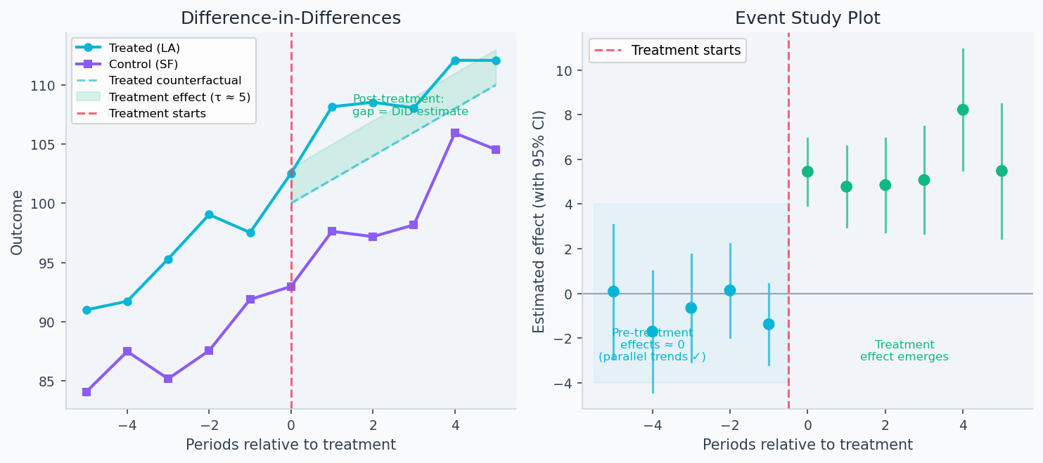
The left panel below shows DiD in action: LA and SF track each other closely before the launch (parallel trends holds), then LA diverges post-treatment while SF continues on the same trajectory — the gap is the causal estimate. The right panel shows an event study: pre-treatment coefficients all near zero validate parallel trends, while post-treatment coefficients reveal the treatment effect emerging and persisting.

Difference-in-Differences and event study plot

With panel data (multiple time periods), estimate using two-way fixed effects (unit fixed effects $\alpha_i$ absorb time-invariant unit differences; time fixed effects $\lambda_t$ absorb common shocks):

$Y_{it} = \alpha_i + \lambda_t + \tau \cdot \text{Treated}_i \cdot \text{Post}_t + \varepsilon_{it}$

Regression Discontinuity (RDD)

RDD exploits a threshold rule: units with running variable $X > c$ receive treatment, units below don't. Near the cutoff $c$ , assignment is "as good as random" — units just above and just below differ only in treatment status.

$\hat{\tau}_{\text{RDD}} = \lim_{x \downarrow c} E[Y \mid X=x] - \lim_{x \uparrow c} E[Y \mid X=x]$

Example: Users with ≥10 lifetime purchases get access to a loyalty program. A user with exactly 10 purchases is nearly identical to one with 9, except one qualifies.

The identifying assumption is continuity: all other determinants of $Y$ (other than treatment) vary continuously at $c$ . A discontinuity in user density at $c$ (McCrary test) suggests users are manipulating their score to cross the threshold — violating continuity.

RDD identifies treatment effect only at the cutoff — the estimate cannot be extrapolated to units far from $c$ . This is both a weakness (external validity) and a strength (the comparison group is maximally credible near the threshold).

Instrumental Variables (IV)

IV handles unobserved confounders by exploiting an instrument $Z$ that satisfies:

Relevance: $Z$ affects treatment $T$ (testable: first-stage F-statistic)
Exclusion restriction: $Z$ affects outcome $Y$ only through $T$ (untestable)
Independence: $Z$ is as-good-as-randomly-assigned (often justifiable by design)

Example: You want to know the effect of daily usage $T$ on 6-month retention $Y$ . Engagement and retention are both caused by unobserved "user fit." The instrument: whether the user received a tutorial email during onboarding (randomly sent to 50%).

The IV estimand is the Local Average Treatment Effect (LATE) — the ATE among compliers: users whose treatment changed because of the instrument. If 30% of users changed their usage because of the email, LATE applies to those 30%.

$\hat{\tau}_{\text{IV}} = \frac{\text{Cov}(Y, Z)}{\text{Cov}(T, Z)} = \frac{E[Y \mid Z=1] - E[Y \mid Z=0]}{E[T \mid Z=1] - E[T \mid Z=0]}$

Two-Stage Least Squares (2SLS) extends this to multiple instruments and controls: $\hat{T}_i = \hat{\pi}_0 + \hat{\pi}_1 Z_i + \hat{\pi}_2 X_i \quad \text{(first stage)}$ $Y_i = \hat{\alpha} + \hat{\tau}_{2\text{SLS}} \hat{T}_i + \hat{\beta} X_i + \varepsilon_i \quad \text{(second stage)}$

Walkthrough

DiD with event study

python

import pandas as pd
import statsmodels.formula.api as smf
 
def run_did(df: pd.DataFrame) -> dict:
    """
    Two-way fixed effects DiD.
    df columns: outcome, treated (unit-level 0/1), post (0/1), unit_id, time
    Clustered standard errors at unit level.
    """
    model = smf.ols(
        "outcome ~ treated:post + C(unit_id) + C(time)",
        data=df
    ).fit(cov_type='cluster', cov_kwds={'groups': df['unit_id']})
 
    return {
        "ate": model.params['treated:post'],
        "se": model.bse['treated:post'],
        "p_value": model.pvalues['treated:post'],
        "ci_95": model.conf_int().loc['treated:post'].tolist(),
    }
 
def run_event_study(df: pd.DataFrame, treatment_period: int) -> pd.DataFrame:
    """
    Event study: estimate per-period effects to test parallel trends pre-treatment
    and reveal treatment dynamics post-treatment.
    Pre-treatment estimates near zero → parallel trends likely holds.
    """
    df = df.copy()
    df['rel_time'] = df['period'] - treatment_period
 
    for k in sorted(df['rel_time'].unique()):
        if k != -1:  # period -1 is the omitted baseline
            df[f'evt_{k}'] = (df['rel_time'] == k) * df['treated']
 
    evt_cols = [c for c in df.columns if c.startswith('evt_')]
    model = smf.ols(
        f"outcome ~ {' + '.join(evt_cols)} + C(unit_id) + C(period)",
        data=df
    ).fit(cov_type='cluster', cov_kwds={'groups': df['unit_id']})
 
    results = []
    for col in evt_cols:
        k = int(col.replace('evt_', ''))
        results.append({
            'rel_time': k,
            'estimate': model.params[col],
            'ci_lower': model.conf_int().loc[col, 0],
            'ci_upper': model.conf_int().loc[col, 1],
            'p_value': model.pvalues[col],
            'is_pre': k < 0,
        })
 
    return pd.DataFrame(results).sort_values('rel_time')
 
# Parallel trends check
event_study = run_event_study(df, treatment_period=10)
pre = event_study[event_study['is_pre']]
print("Pre-treatment effects (should all be near zero):")
print(pre[['rel_time', 'estimate', 'p_value']])

RDD with McCrary density test

python

import numpy as np
from sklearn.linear_model import LinearRegression
 
def rdd_local_linear(
    scores: np.ndarray,
    outcomes: np.ndarray,
    cutoff: float,
    bandwidth: float,
) -> dict:
    """
    Local linear RDD estimator.
    Fits separate linear regressions on each side; treatment effect = discontinuity at cutoff.
    """
    mask = np.abs(scores - cutoff) <= bandwidth
    X_c = scores[mask] - cutoff  # centered running variable
    Y = outcomes[mask]
    treated = (X_c >= 0).astype(float)
 
    X_mat = np.column_stack([treated, X_c, treated * X_c])
    model = LinearRegression().fit(X_mat, Y)
    tau = model.coef_[0]
 
    # Bootstrap SE
    n = mask.sum()
    boot_taus = []
    for _ in range(500):
        idx = np.random.choice(n, n, replace=True)
        m = LinearRegression().fit(X_mat[idx], Y[idx])
        boot_taus.append(m.coef_[0])
 
    se = np.std(boot_taus)
    return {
        "ate_at_cutoff": round(tau, 4),
        "se": round(se, 4),
        "ci_95": (round(tau - 1.96*se, 4), round(tau + 1.96*se, 4)),
        "n_in_bandwidth": int(n),
        "bandwidth": bandwidth,
    }
 
def mccrary_density_test(
    scores: np.ndarray,
    cutoff: float,
    bandwidth: float,
) -> dict:
    """
    McCrary density test: checks if the running variable density is continuous at the cutoff.
    A discontinuity suggests users manipulated their score to receive treatment.
    """
    bin_width = bandwidth / 10
    bins = np.arange(cutoff - bandwidth, cutoff + bandwidth + bin_width, bin_width)
    counts, edges = np.histogram(scores, bins=bins)
    centers = (edges[:-1] + edges[1:]) / 2 - cutoff
    density = counts / (len(scores) * bin_width)
 
    def fit_intercept(x, y):
        X_mat = np.column_stack([np.ones_like(x), x])
        coef = np.linalg.lstsq(X_mat, y, rcond=None)[0]
        return coef[0]
 
    d_left = fit_intercept(centers[centers < 0], density[centers < 0])
    d_right = fit_intercept(centers[centers >= 0], density[centers >= 0])
 
    jump_pct = abs(d_right - d_left) / max(d_left, 1e-10)
    return {
        "density_left": round(d_left, 5),
        "density_right": round(d_right, 5),
        "jump_pct": round(jump_pct, 3),
        "manipulation_flag": jump_pct > 0.10,
    }

IV with weak instrument test

python

import statsmodels.formula.api as smf
from scipy import stats
from linearmodels.iv import IV2SLS
 
def check_instrument_strength(
    df: pd.DataFrame,
    treatment: str,
    instrument: str,
    controls: list = None,
) -> dict:
    """
    First-stage F-statistic for instrument relevance.
    Rule: F > 16.38 for 10% worst-case 2SLS bias (Stock-Yogo, 1 instrument).
    The common "F > 10" threshold is too lenient.
    """
    ctrl = ' + '.join(controls) if controls else '1'
    model_full = smf.ols(f"{treatment} ~ {instrument} + {ctrl}", data=df).fit()
    model_restr = smf.ols(f"{treatment} ~ {ctrl}", data=df).fit()
 
    n, k = len(df), (len(controls) if controls else 0) + 1
    f_stat = ((model_restr.ssr - model_full.ssr)) / (model_full.ssr / (n - k - 1))
    p_val = 1 - stats.f.cdf(f_stat, 1, n - k - 1)
 
    return {
        "first_stage_coef": round(model_full.params[instrument], 4),
        "f_statistic": round(f_stat, 2),
        "p_value": round(p_val, 6),
        "strength": "strong" if f_stat > 16.38 else "moderate" if f_stat > 10 else "weak (biased 2SLS)",
    }
 
def run_iv_2sls(df: pd.DataFrame) -> dict:
    """Two-stage least squares via linearmodels."""
    result = IV2SLS(
        dependent=df['retention_6m'],
        endog=df['daily_usage'],
        exog=df[['const', 'age', 'platform']],
        instruments=df['received_tutorial_email'],
    ).fit()
 
    return {
        "late": round(result.params['daily_usage'], 4),
        "se": round(result.std_errors['daily_usage'], 4),
        "ci_95": tuple(round(x, 4) for x in result.conf_int().loc['daily_usage']),
        "p_value": round(result.pvalues['daily_usage'], 5),
        "interpretation": "LATE: effect on compliers only",
    }

Analysis & Evaluation

Where Your Intuition Breaks

More pre-treatment periods make DiD more reliable. Pre-treatment data validates the parallel trends assumption by showing the groups tracked each other historically — but parallel pre-trends is a necessary condition, not a sufficient one. Two groups can trend together for years and diverge post-treatment for reasons unrelated to the intervention (a simultaneous policy change, an economic shock that affected them differently). Pre-trend tests reduce skepticism; they do not establish causality. The parallel trends assumption is fundamentally about the counterfactual post-period, which is unobservable regardless of how clean the pre-period looks.

When each method applies

Situation	Method	Key assumption
Treated group has a comparable control group, pre-post data available	Difference-in-Differences	Parallel trends
Eligibility determined by crossing a threshold	Regression Discontinuity	Continuity at cutoff
Treatment has unobserved causes, valid instrument exists	Instrumental Variables	Exclusion restriction + relevance

DiD assumption testing:

Plot pre-treatment time series for treated and control — should be parallel
Event study: pre-treatment coefficients should be near zero
Falsification: test on outcomes that shouldn't be affected by treatment

RDD assumption testing:

McCrary test: density of running variable should be continuous at cutoff
Covariate continuity: pre-treatment covariates should not jump at cutoff
Bandwidth sensitivity: re-run with 0.5x and 2x bandwidth; estimates should be stable

IV assumption testing:

Relevance: F-statistic > 16.38 (Stock-Yogo threshold)
Exclusion: economic argument (cannot be tested statistically)
Independence: can check by regressing instrument on observed confounders — should be insignificant

LATE vs. ATE: does it matter?

IV estimates LATE — the effect on compliers. Compliers are the subpopulation whose treatment status changed because of the instrument. Three other populations exist:

Always-takers: $T=1$ regardless of $Z$
Never-takers: $T=0$ regardless of $Z$
Defiers: $T=1$ when $Z=0$ , $T=0$ when $Z=1$ (excluded by monotonicity assumption)

If the tutorial email (instrument) only affects casual users (the marginal user who needs a nudge), the LATE is the effect of engagement on casual users — which may not generalize to heavy users. Whether LATE is the right estimand depends on your policy question.

⚠️Warning

DiD with staggered treatment timing (different units treated at different times) cannot use the standard two-way fixed effects estimator — recent econometrics work (Callaway and Sant'Anna, 2021; Goodman-Bacon, 2021) shows it can produce severely biased estimates when treatment effects are heterogeneous across cohorts. Use estimators designed for staggered adoption when your treatment timing varies across units.

Staggered rollouts as natural experiments

A phased product rollout — Week 1: 5 cities, Week 2: 15 cities, Week 3: all cities — creates natural DiD variation. Each city that gets the feature becomes treated; others serve as controls until they're treated.

With staggered timing, use the Callaway-Sant'Anna estimator (implemented in the csdid Python package) rather than standard two-way fixed effects:

python

# Pseudocode — exact syntax depends on csdid package version
from csdid import att_gt
 
# att_gt computes the ATT for each (group, time) pair
# where group = the first period when the unit is treated
att_results = att_gt(
    yname="outcome",
    gname="first_treat",    # period when unit was first treated (0 if never)
    idname="unit_id",
    tname="period",
    data=df,
    control_group="notyettreated",  # use not-yet-treated units as controls
)
 
# Aggregate to overall ATT
overall_att = att_results.aggte(type="simple")
print(f"Overall ATT: {overall_att.overall_att:.4f} (SE: {overall_att.se:.4f})")

🚀Production

When launching host-side features (which violate SUTVA at the user level), city-level DiD is a common approach: treat some cities, leave others as controls, compare revenue trends. The key challenge is finding control cities with genuinely parallel pre-treatment trends. A combination of event study plots and synthetic control (to construct a better counterfactual than any single city) validates the assumption before trusting the estimate.

Production-Ready Code

A production DiD pipeline pre-tests parallel trends before computing the estimate — a trend violation at p < 0.10 is a warning that the control group may not be a valid counterfactual. The event study view is more informative than the single DiD scalar: it shows when the effect emerged, whether it persisted, and whether pre-trends were truly flat.

python

# production_quasi_experimental.py
# DiD pipeline with parallel trends pre-test and event study.
 
from __future__ import annotations
import numpy as np
import pandas as pd
import scipy.stats as stats
 
 
def did_pipeline(
    df: pd.DataFrame,
    outcome: str,
    treated_unit: str,
    unit_col: str,
    time_col: str,
    treat_period: int,
) -> dict:
    """
    Two-way fixed effects DiD with parallel trends pre-test.
    Returns the DiD estimate, SE, p-value, and parallel trends verdict.
    """
    df = df.copy()
    df["_treated"] = (df[unit_col] == treated_unit).astype(float)
    df["_post"]    = (df[time_col] >= treat_period).astype(float)
    df["_did"]     = df["_treated"] * df["_post"]
 
    # Simple DiD scalar from 2x2 means
    m = df.groupby(["_treated", "_post"])[outcome].mean()
    tau = (m[1.0, 1.0] - m[1.0, 0.0]) - (m[0.0, 1.0] - m[0.0, 0.0])
 
    # OLS with unit + time dummies for SE
    units = pd.get_dummies(df[unit_col], prefix="u", drop_first=True)
    times = pd.get_dummies(df[time_col], prefix="t", drop_first=True)
    X = pd.concat([df[["_did"]], units, times], axis=1).astype(float).values
    y = df[outcome].values
    coef, *_ = np.linalg.lstsq(X, y, rcond=None)
    resid = y - X @ coef
    n, k = len(y), X.shape[1]
    sigma2 = (resid ** 2).sum() / (n - k)
    se = float(np.sqrt(sigma2 * np.linalg.pinv(X.T @ X)[0, 0]))
    t_stat = float(coef[0] / se)
    p_val  = float(2 * (1 - stats.t.cdf(abs(t_stat), df=n - k)))
 
    # Parallel trends pre-test: time x treated interaction in pre-period
    pre = df[df["_post"] == 0].copy()
    pre["_time"] = pre[time_col] - pre[time_col].min()
    pre["_inter"] = pre["_time"] * pre["_treated"]
    Xp = np.column_stack([
        np.ones(len(pre)), pre["_time"].values,
        pre["_treated"].values, pre["_inter"].values,
    ])
    cp, *_ = np.linalg.lstsq(Xp, pre[outcome].values, rcond=None)
    resid_p = pre[outcome].values - Xp @ cp
    np_, kp = len(pre), 4
    s2p = (resid_p ** 2).sum() / (np_ - kp)
    se_inter = float(np.sqrt(s2p * np.linalg.pinv(Xp.T @ Xp)[3, 3]))
    t_inter = cp[3] / se_inter
    p_inter = float(2 * (1 - stats.t.cdf(abs(t_inter), df=np_ - kp)))
 
    return {
        "tau_did": round(float(tau), 5),
        "tau_se": round(se, 5),
        "tau_p": round(p_val, 6),
        "significant": p_val < 0.05,
        "parallel_trends": {
            "interaction_coef": round(float(cp[3]), 5),
            "p_value": round(p_inter, 6),
            "holds": p_inter > 0.10,
            "verdict": "OK — consistent with parallel trends"
            if p_inter > 0.10
            else "WARNING — pre-trends differ; DiD estimate may be biased",
        },
    }
 
 
def event_study(
    df: pd.DataFrame,
    outcome: str,
    treated_unit: str,
    unit_col: str,
    time_col: str,
    treat_period: int,
) -> pd.DataFrame:
    """
    Per-period treatment coefficients relative to treat_period - 1 (omitted).
    Pre-period coefficients near zero validate parallel trends visually.
    """
    df = df.copy()
    df["_treated"] = (df[unit_col] == treated_unit).astype(float)
    ref = treat_period - 1
    rows = []
    for t in sorted(df[time_col].unique()):
        if t == ref:
            continue
        sub = df[df[time_col] == t]
        effect = (
            sub.loc[sub["_treated"] == 1, outcome].mean()
            - sub.loc[sub["_treated"] == 0, outcome].mean()
        )
        rows.append({"period": t, "relative_period": t - treat_period, "effect": round(effect, 5)})
    return pd.DataFrame(rows)
 
 
# ── Example ───────────────────────────────────────────────────────────────────
rng = np.random.default_rng(42)
periods = list(range(2020, 2026))
units   = ["LA", "SF", "NYC", "CHI", "SEA"]
records = []
for unit in units:
    for t in periods:
        base = rng.normal(100, 5)
        treat_effect = 8.0 if (unit == "LA" and t >= 2023) else 0.0
        records.append({
            "city": unit, "year": t,
            "revenue": base + (t - 2020) * 2 + treat_effect + rng.normal(0, 2),
        })
df = pd.DataFrame(records)
print(did_pipeline(df, "revenue", "LA", "city", "year", treat_period=2023))
print(event_study(df, "revenue", "LA", "city", "year", treat_period=2023))

Enjoying these notes?

Get new lessons delivered to your inbox. No spam.

Potential Outcomes & DAGs

Propensity Scores & Modern Methods