Requires:Quasi-Experimental Methods

Propensity Scores & Modern Methods

When you have rich observational data and believe you've measured all relevant confounders, propensity scores collapse the high-dimensional matching problem into a single scalar: the probability a unit would have been treated given its covariates. Weighting by inverse propensity recreates the equivalent of a randomized experiment from observational data — but only if the weights are well-behaved. Double ML extends this to the case where hundreds of features need to be controlled for, using cross-fitting to avoid regularization bias on the treatment effect estimate. Synthetic control handles the case where the treatment is a single unit (a city, a country, a product line) by constructing a weighted combination of control units that best matches its pre-treatment history. Each method handles a different regime of the observational inference problem, and each fails in a different way when its assumptions are violated — which is why sensitivity analysis (Rosenbaum bounds) is not optional.

Theory

Love Plot — Covariate Balance

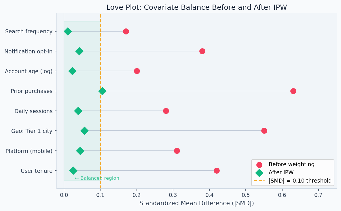
Each row is one covariate. After propensity score weighting, all SMDs fall inside ±0.1 (dashed lines) — treated and control groups are now comparable on observables.

In an observational study, treated and control units differ not just in treatment but in everything that made them more or less likely to be treated. Older patients get more aggressive treatment; wealthier customers get premium products. The propensity score compresses all those confounders into a single number — the probability of treatment — making it possible to compare units with the same probability of being treated but different actual assignments.

Propensity scores

When you have rich observational data and believe unconfoundedness holds — all confounders are measured — propensity scores provide a dimensionality reduction for causal estimation.

The propensity score is: $e(X_i) = P(T_i = 1 \mid X_i)$

The propensity score works as a sufficient statistic for the full covariate vector because the balancing property is a consequence of probability theory, not an additional assumption. If two units have the same $e(x)$ , their covariate distributions are identical in expectation — so any remaining difference in outcomes between treated and control units at that propensity score level must reflect the treatment effect, not selection bias. This is what makes a scalar summary of all confounders sufficient for identification, even when the covariate space is high-dimensional.

Balancing score theorem (Rosenbaum and Rubin, 1983): conditioning on $e(X_i)$ balances the full covariate vector $X_i$ between treated and control groups:

$T_i \perp\!\!\!\perp X_i \mid e(X_i)$

Combined with unconfoundedness $(Y_i(t) \perp\!\!\!\perp T_i \mid X_i)$ , this gives: $Y_i(t) \perp\!\!\!\perp T_i \mid e(X_i)$

You only need to condition on a scalar $e(x)$ rather than the full covariate vector — a dramatic simplification, especially in high dimensions.

Overlap assumption: for propensity score methods to work, every unit must have a positive probability of both treatment and control: $0 < e(X_i) < 1 \quad \text{for all } X_i$

Violations create extreme weights ( $1/e(x) \to \infty$ ), inflating variance. Trim units with $e(x) < \epsilon$ or $e(x) > 1-\epsilon$ (common: $\epsilon = 0.05$ ). This buys variance reduction at the cost of external validity (you're excluding non-comparable units).

Inverse Probability Weighting (IPW)

IPW reweights the observed sample to make it representative of the target population. The Horvitz-Thompson estimator:

$\hat{\tau}_{\text{IPW}} = \frac{1}{n}\sum_{i=1}^n \left[\frac{T_i Y_i}{e(X_i)} - \frac{(1-T_i)Y_i}{1-e(X_i)}\right]$

For treated units: weight $1/e(X_i)$ — rare treated units (low $e(x)$ ) get high weight, making them represent the full population. For control units: weight $1/(1-e(X_i))$ .

IPW is consistent when the propensity score model is correct. But it is sensitive to model misspecification — a slightly wrong model produces extreme weights and high-variance estimates.

After fitting IPW weights, the standard diagnostic is a Love plot — standardized mean differences (SMD) for each covariate before and after weighting. Values below |SMD| = 0.10 indicate good balance. The figure below shows what successful IPW looks like: pre-weighting SMDs as high as 0.63 on "prior purchases" collapse to near zero post-weighting across all features.

Love plot showing covariate balance before and after IPW

Doubly robust estimation

The doubly robust (DR) estimator combines IPW with outcome regression. It is consistent if either the propensity score model or the outcome model is correctly specified — not necessarily both.

$\hat{\tau}_{\text{DR}} = \frac{1}{n}\sum_{i=1}^n \underbrace{\left[\frac{T_i(Y_i - \hat{\mu}_1(X_i))}{\hat{e}(X_i)} - \frac{(1-T_i)(Y_i - \hat{\mu}_0(X_i))}{1-\hat{e}(X_i)}\right]}_{\text{IPW residual}} + \underbrace{(\hat{\mu}_1(X_i) - \hat{\mu}_0(X_i))}_{\text{outcome regression}}$

When the outcome models $\hat{\mu}_t(x) = E[Y \mid T=t, X=x]$ are correct, the IPW residual terms have expectation zero — the estimator is just the outcome regression part. When the propensity score is correct, the IPW residuals correct for any outcome model misspecification. The two models "doubly protect" each other.

Double Machine Learning

Double Machine Learning (Double ML) (Chernozhukov et al., 2018) handles high-dimensional confounders via Neyman orthogonality. The idea: residualize both $Y$ and $T$ on $X$ using flexible ML, then regress the residuals on each other.

Step 1 (cross-fitting): on held-out folds, estimate: $\tilde{Y}_i = Y_i - \hat{m}(X_i), \quad \tilde{T}_i = T_i - \hat{e}(X_i)$

Step 2: regress $\tilde{Y}$ on $\tilde{T}$ : $\hat{\tau} = \frac{\sum_i \tilde{T}_i \tilde{Y}_i}{\sum_i \tilde{T}_i^2}$

The Neyman orthogonality condition ensures that nuisance estimation errors enter the score only at second order — so $\hat{\tau}$ is $\sqrt{n}$ -consistent even when $\hat{m}$ and $\hat{e}$ converge at slower rates (e.g., $n^{-1/4}$ ). This is the key advantage over naive plug-in estimation.

Synthetic Control

When there is only one treated unit (a country, a product line, a city) and several potential controls, synthetic control constructs a weighted combination of controls that matches the treated unit's pre-treatment trajectory:

$Y_{\text{synthetic}} = \sum_{j=1}^{J} w_j Y_j, \quad w_j \geq 0, \quad \sum_j w_j = 1$

Weights are chosen to minimize pre-treatment fit. Post-treatment, the synthetic control is the counterfactual. The treatment effect is the gap between the treated unit and its synthetic version.

Inference via placebo tests: with one treated unit, classical standard errors don't apply. Apply the same synthetic control procedure to each donor unit (as if it were treated). The p-value is the fraction of donors whose post/pre MSPE ratio exceeds the treated unit's.

Rosenbaum sensitivity analysis

After finding a significant effect from an observational study, how robust is it to unobserved confounding? Rosenbaum bounds quantify this.

Allow two matched units with identical observed covariates to differ in treatment odds by at most $\Gamma$ : $\frac{1}{\Gamma} \leq \frac{\text{odds}(T_i=1 \mid X_i)}{\text{odds}(T_j=1 \mid X_j)} \leq \Gamma$

At $\Gamma = 1$ : no hidden bias. For each $\Gamma$ , compute the worst-case p-value. The sensitivity threshold $\Gamma^*$ is the smallest $\Gamma$ that overturns your conclusion.

$\Gamma^* = 1.5$ means: a confounder that multiplied treatment odds by 1.5 would make the result insignificant. $\Gamma^* = 3.0$ means: you'd need a confounder tripling the treatment odds to explain away the effect. Large $\Gamma^*$ → robust result.

Walkthrough

Doubly robust ATE with cross-fitting

python

import numpy as np
from sklearn.ensemble import GradientBoostingClassifier, GradientBoostingRegressor
from sklearn.model_selection import KFold, cross_val_predict
from scipy import stats
 
def doubly_robust_ate(
    X: np.ndarray,
    T: np.ndarray,
    Y: np.ndarray,
    n_folds: int = 5,
) -> dict:
    """
    Doubly robust ATE with cross-fitting.
    Cross-fitting prevents nuisance model overfitting from biasing the ATE estimate.
    """
    n = len(Y)
 
    # Cross-fit propensity score e(X) = P(T=1 | X)
    ps_model = GradientBoostingClassifier(n_estimators=100, max_depth=3, random_state=42)
    e_hat = cross_val_predict(ps_model, X, T, cv=n_folds, method='predict_proba')[:, 1]
    e_hat = np.clip(e_hat, 0.05, 0.95)  # Trim extreme weights
 
    # Cross-fit outcome models mu_1(X) = E[Y|T=1,X] and mu_0(X) = E[Y|T=0,X]
    mu1_hat = np.zeros(n)
    mu0_hat = np.zeros(n)
 
    kf = KFold(n_splits=n_folds, shuffle=True, random_state=42)
    for train_idx, val_idx in kf.split(X):
        X_tr, T_tr, Y_tr = X[train_idx], T[train_idx], Y[train_idx]
        m1 = GradientBoostingRegressor(n_estimators=100, random_state=42)
        m0 = GradientBoostingRegressor(n_estimators=100, random_state=42)
        m1.fit(X_tr[T_tr == 1], Y_tr[T_tr == 1])
        m0.fit(X_tr[T_tr == 0], Y_tr[T_tr == 0])
        mu1_hat[val_idx] = m1.predict(X[val_idx])
        mu0_hat[val_idx] = m0.predict(X[val_idx])
 
    # Doubly robust scores
    dr_scores = (
        T * (Y - mu1_hat) / e_hat
        - (1 - T) * (Y - mu0_hat) / (1 - e_hat)
        + mu1_hat - mu0_hat
    )
 
    tau = dr_scores.mean()
    se = dr_scores.std() / np.sqrt(n)
    return {
        "ate": round(tau, 4),
        "se": round(se, 4),
        "ci_95": (round(tau - 1.96*se, 4), round(tau + 1.96*se, 4)),
        "p_value": round(2 * (1 - stats.norm.cdf(abs(tau/se))), 5),
    }

Propensity score diagnostics

Before interpreting any propensity score estimate, verify that the model achieves covariate balance. The standardized mean difference (SMD) should be below 0.1 for all covariates after weighting:

$\text{SMD}_k = \frac{\bar{X}_{k,\text{treated}} - \bar{X}_{k,\text{control}}}{\sqrt{(s_{k,\text{treated}}^2 + s_{k,\text{control}}^2)/2}}$

python

import pandas as pd
import numpy as np
 
def compute_smd(
    df: pd.DataFrame,
    covariates: list,
    treatment_col: str,
    weights: np.ndarray = None,
) -> pd.DataFrame:
    """Standardized mean differences before/after IPW weighting."""
    treated = df[treatment_col] == 1
    control = df[treatment_col] == 0
    results = []
 
    for cov in covariates:
        x_t = df.loc[treated, cov].values
        x_c = df.loc[control, cov].values
        pooled_sd = np.sqrt((x_t.var() + x_c.var()) / 2 + 1e-10)
        smd_raw = (x_t.mean() - x_c.mean()) / pooled_sd
 
        smd_w = None
        if weights is not None:
            w_t, w_c = weights[treated.values], weights[control.values]
            smd_w = (np.average(x_t, weights=w_t) - np.average(x_c, weights=w_c)) / pooled_sd
 
        results.append({
            'covariate': cov,
            'smd_raw': round(smd_raw, 3),
            'smd_weighted': round(smd_w, 3) if smd_w is not None else None,
            'balanced': abs(smd_w or smd_raw) < 0.1,
        })
 
    return pd.DataFrame(results).sort_values('smd_raw', key=abs, ascending=False)
 
# Compute IPW weights and check balance
from sklearn.linear_model import LogisticRegression
ps = LogisticRegression(max_iter=500).fit(X, T)
e_hat = ps.predict_proba(X)[:, 1]
ipw_weights = np.where(T == 1, 1/e_hat, 1/(1-e_hat))
 
smd = compute_smd(df, covariates, 'treated', weights=ipw_weights)
print(smd)
# Aim for all |smd_weighted| < 0.1 before trusting the IPW estimate

Synthetic control with placebo inference

python

from scipy.optimize import minimize
import numpy as np
 
def synthetic_control(
    Y_treated: np.ndarray,
    Y_donors: np.ndarray,
    T0: int,
) -> dict:
    """
    Synthetic control: find donor weights minimizing pre-treatment fit.
    T0: number of pre-treatment periods.
    """
    y_pre, X_pre = Y_treated[:T0], Y_donors[:T0]
    J = X_pre.shape[1]
 
    result = minimize(
        lambda w: np.sum((y_pre - X_pre @ w)**2),
        x0=np.ones(J)/J,
        bounds=[(0, 1)]*J,
        constraints={'type': 'eq', 'fun': lambda w: w.sum() - 1},
    )
    w = result.x
    y_synth = Y_donors @ w
    effects = Y_treated[T0:] - y_synth[T0:]
 
    return {
        "weights": w,
        "y_synthetic": y_synth,
        "att": effects.mean(),
        "pre_fit_rmse": float(np.sqrt(np.mean((y_pre - y_synth[:T0])**2))),
        "post_effects": effects,
    }
 
def placebo_p_value(
    Y_treated: np.ndarray,
    Y_donors: np.ndarray,
    T0: int,
) -> float:
    """
    Placebo inference: apply synthetic control to each donor unit.
    P-value = fraction of donors with larger post/pre MSPE ratio than the treated unit.
    """
    def mspe_ratio(y_unit, y_other, T0):
        r = synthetic_control(y_unit, y_other, T0)
        pre_mspe = np.mean((y_unit[:T0] - r['y_synthetic'][:T0])**2)
        post_mspe = np.mean((y_unit[T0:] - r['y_synthetic'][T0:])**2)
        return post_mspe / (pre_mspe + 1e-10)
 
    J = Y_donors.shape[1]
    treated_ratio = mspe_ratio(Y_treated, Y_donors, T0)
 
    # Placebo: treat each donor as if it were the treated unit
    placebo_ratios = []
    for j in range(J):
        other_donors = np.delete(Y_donors, j, axis=1)
        r = mspe_ratio(Y_donors[:, j], other_donors, T0)
        placebo_ratios.append(r)
 
    p_val = np.mean(np.array(placebo_ratios) >= treated_ratio)
    return round(p_val, 3)

Rosenbaum sensitivity bounds

python

from scipy import stats
 
def rosenbaum_sensitivity(
    treated_outcomes: np.ndarray,
    control_outcomes: np.ndarray,
    gamma_range: list = None,
) -> pd.DataFrame:
    """
    Sensitivity analysis for matched pairs under Rosenbaum's model.
    gamma_range: list of Gamma values to test.
    """
    if gamma_range is None:
        gamma_range = [1.0, 1.25, 1.5, 2.0, 2.5, 3.0]
 
    diffs = treated_outcomes - control_outcomes
    n = len(diffs)
    ranks = stats.rankdata(np.abs(diffs))
    T_obs = sum(r for r, d in zip(ranks, diffs) if d > 0)
 
    rows = []
    for gamma in gamma_range:
        p_plus = gamma / (1 + gamma)
        E_T = n*(n+1)/2 * p_plus
        Var_T = n*(n+1)*(2*n+1)/6 * p_plus*(1-p_plus)
        z = (T_obs - E_T) / np.sqrt(Var_T)
        p_worst = 1 - stats.norm.cdf(z)
        rows.append({
            'gamma': gamma,
            'p_worst_case': round(p_worst, 5),
            'conclusion_holds': p_worst < 0.05,
        })
 
    return pd.DataFrame(rows)
 
# Interpret: find gamma* — the smallest Gamma where conclusion_holds = False
# gamma*=1.5 → fragile; gamma*=3.0 → robust to large hidden confounders

Analysis & Evaluation

Where Your Intuition Breaks

A good Love plot (balanced covariates after weighting) means the causal estimate is valid. Covariate balance is a necessary condition for unconfoundedness, not a sufficient one. A Love plot only shows balance on measured covariates — unmeasured confounders remain unbalanced regardless of how well the propensity model performs on observed features. Rosenbaum sensitivity analysis quantifies how large an unmeasured confounder would need to be to reverse the conclusion, but it cannot rule out confounding. Perfect balance on observables with a hidden confounder still produces a biased estimate.

Method selection guide

Situation	Method	Identifying assumption
Random assignment possible	RCT	None
Phased rollout / regional variation	DiD	Parallel trends
Threshold-based eligibility	RDD	Continuity at cutoff
Valid instrument available	IV / 2SLS	Exclusion restriction
Single treated unit	Synthetic Control	Pre-treatment fit
Rich covariates, unconfoundedness plausible	DR / Double ML	No unmeasured confounders

When multiple methods are available, triangulate. If DiD, IV, and doubly robust all give similar estimates, that's much stronger evidence than any single method alone.

Assumption severity

Not all identifying assumptions are equally testable or plausible:

Assumption	Testable?	Severity if violated
Parallel trends (DiD)	Partially (pre-period)	Moderate — can add unit trends
Continuity (RDD)	Yes (McCrary, covariate continuity)	Severe — invalidates RDD entirely
Exclusion restriction (IV)	No — requires economic reasoning	Severe — biases 2SLS toward OLS
No unmeasured confounders	No — requires domain knowledge	Severe — quantify with Rosenbaum bounds
Overlap (PS methods)	Yes — check propensity score distribution	Moderate — trim and note external validity loss

⚠️Warning

Causal inference from observational data is not as reliable as a randomized experiment. Observational estimates carry implicit assumptions that cannot be verified from data alone. When you report an observational effect, always state which assumption you're relying on, how you've tried to validate it, and what a Rosenbaum sensitivity analysis says about robustness.

End-to-end observational pipeline

python

from dataclasses import dataclass, field
 
@dataclass
class CausalResult:
    method: str
    ate: float
    ci_lower: float
    ci_upper: float
    p_value: float
    n_units: int
    validated: dict = field(default_factory=dict)
    warnings: list = field(default_factory=list)
 
def observational_pipeline(df, outcome, treatment, covariates):
    """Standard pipeline: overlap check → balance check → DR estimation → validation."""
    warnings, validated = [], {}
    X, T, Y = df[covariates].values, df[treatment].values, df[outcome].values
 
    # 1. Fit propensity score and check overlap
    from sklearn.linear_model import LogisticRegression
    ps = LogisticRegression(max_iter=500).fit(X, T)
    e_hat = ps.predict_proba(X)[:, 1]
    poor_overlap = ((e_hat < 0.05) | (e_hat > 0.95)).mean()
    if poor_overlap > 0.05:
        warnings.append(f"Overlap: {poor_overlap:.1%} of units outside [0.05, 0.95]")
    validated['overlap'] = poor_overlap < 0.05
 
    # 2. Pre-treatment balance
    smd = compute_smd(df, covariates, treatment)
    max_smd = smd['smd_raw'].abs().max()
    if max_smd > 0.25:
        warnings.append(f"High pre-treatment imbalance: max SMD = {max_smd:.2f}")
 
    # 3. Doubly robust ATE
    res = doubly_robust_ate(X, T, Y)
 
    # 4. Post-weighting balance check
    ipw_w = np.where(T == 1, 1/e_hat, 1/(1-e_hat))
    smd_after = compute_smd(df, covariates, treatment, weights=ipw_w)
    max_smd_after = smd_after['smd_weighted'].abs().max()
    validated['balance'] = max_smd_after < 0.1
    if max_smd_after >= 0.1:
        warnings.append(f"Post-weighting imbalance: max SMD = {max_smd_after:.2f}")
 
    return CausalResult(
        method="doubly_robust",
        ate=res['ate'], ci_lower=res['ci_95'][0], ci_upper=res['ci_95'][1],
        p_value=res['p_value'], n_units=len(df),
        validated=validated, warnings=warnings,
    )

🚀Production

In platforms where A/B tests can't be run (supply-side features, city-level policy changes), causal inference from observational data is the only option. Best practice: run at least two independent methods (e.g., DiD and synthetic control), plot event study diagnostics to validate parallel trends, and report Rosenbaum bounds alongside the estimate. An observational result that hasn't been validated with multiple methods should be treated as exploratory and not used for product decisions.

Production-Ready Code

Doubly-robust AIPW is the production-grade default when you have enough covariates to worry about model misspecification. The key operational concern is weight diagnostics: extreme IPW weights signal overlap failures that inflate variance. Cross-fitting is mandatory — in-sample nuisance estimation introduces regularisation bias that contaminates the treatment effect estimate.

python

# production_propensity.py
# AIPW (doubly-robust) ATE estimation with weight diagnostics and overlap trimming.
 
from __future__ import annotations
import math
import numpy as np
import scipy.stats as stats
from sklearn.linear_model import LogisticRegression
from sklearn.ensemble import GradientBoostingRegressor
from sklearn.model_selection import KFold
from sklearn.preprocessing import StandardScaler
 
 
def weight_diagnostics(e_hat: np.ndarray, T: np.ndarray) -> dict:
    """
    Run BEFORE any weighted estimator.
    Extreme weights (max > 20 or ESS < 30% of n) signal overlap failure.
    """
    w = np.where(T == 1, 1.0 / e_hat, 1.0 / (1.0 - e_hat))
    ess = w.sum() ** 2 / (w ** 2).sum()
    return {
        "max_weight":      round(float(w.max()), 2),
        "p99_weight":      round(float(np.percentile(w, 99)), 2),
        "effective_sample_size": round(float(ess), 1),
        "ess_fraction":    round(float(ess / len(T)), 3),
        "min_propensity":  round(float(e_hat.min()), 4),
        "max_propensity":  round(float(e_hat.max()), 4),
        "overlap_warning": bool(e_hat.min() < 0.05 or e_hat.max() > 0.95),
        "action": (
            "Trim units with e < 0.05 or e > 0.95 before weighting"
            if e_hat.min() < 0.05 or e_hat.max() > 0.95
            else "OK"
        ),
    }
 
 
def aipw_ate(
    X: np.ndarray,
    T: np.ndarray,
    Y: np.ndarray,
    n_folds: int = 5,
    trim: float = 0.05,
) -> dict:
    """
    Augmented IPW (doubly-robust) ATE via cross-fitting.
    Doubly robust: consistent if EITHER the propensity OR outcome model is correct.
 
    Cross-fitting removes regularisation bias: nuisance models are trained on
    held-out folds so their errors are orthogonal to the treatment effect estimate.
    """
    n = len(Y)
    scaler = StandardScaler()
    Xs = scaler.fit_transform(X)
    e_hat   = np.zeros(n)
    mu1_hat = np.zeros(n)
    mu0_hat = np.zeros(n)
 
    kf = KFold(n_splits=n_folds, shuffle=True, random_state=42)
    for train_idx, val_idx in kf.split(Xs):
        X_tr, X_val = Xs[train_idx], Xs[val_idx]
        T_tr        = T[train_idx]
        Y_tr        = Y[train_idx]
 
        ps = LogisticRegression(C=1.0, max_iter=500, random_state=42)
        ps.fit(X_tr, T_tr)
        e_hat[val_idx] = ps.predict_proba(X_val)[:, 1]
 
        m1 = GradientBoostingRegressor(n_estimators=100, random_state=42)
        m0 = GradientBoostingRegressor(n_estimators=100, random_state=42)
        if T_tr.sum() >= 10:
            m1.fit(X_tr[T_tr == 1], Y_tr[T_tr == 1])
            mu1_hat[val_idx] = m1.predict(X_val)
        else:
            mu1_hat[val_idx] = Y_tr[T_tr == 1].mean()
        if (1 - T_tr).sum() >= 10:
            m0.fit(X_tr[T_tr == 0], Y_tr[T_tr == 0])
            mu0_hat[val_idx] = m0.predict(X_val)
        else:
            mu0_hat[val_idx] = Y_tr[T_tr == 0].mean()
 
    keep = (e_hat >= trim) & (e_hat <= 1 - trim)
    e_k, mu1_k, mu0_k = e_hat[keep], mu1_hat[keep], mu0_hat[keep]
    T_k, Y_k = T[keep], Y[keep]
 
    psi = (
        T_k * (Y_k - mu1_k) / e_k
        - (1 - T_k) * (Y_k - mu0_k) / (1 - e_k)
        + mu1_k - mu0_k
    )
    tau   = float(psi.mean())
    se    = float(psi.std() / math.sqrt(len(psi)))
    z     = tau / se
    p_val = float(2 * (1 - stats.norm.cdf(abs(z))))
    ci    = (tau - 1.96 * se, tau + 1.96 * se)
 
    return {
        "ate_aipw":      round(tau, 5),
        "se":            round(se, 5),
        "ci_95":         (round(ci[0], 5), round(ci[1], 5)),
        "p_value":       round(p_val, 6),
        "n_trimmed":     int((~keep).sum()),
        "weight_diagnostics": weight_diagnostics(e_hat[keep], T_k),
    }
 
 
# ── Example ───────────────────────────────────────────────────────────────────
rng = np.random.default_rng(42)
n = 2_000
X = rng.normal(0, 1, (n, 5))
propensity = 1 / (1 + np.exp(-X[:, 0]))
T = rng.binomial(1, propensity).astype(float)
Y = 2.5 * T + X[:, 0] + rng.normal(0, 1, n)   # true ATE = 2.5
 
result = aipw_ate(X, T, Y)
print(result)
# ate_aipw ≈ 2.5, overlap_warning: False

Enjoying these notes?

Get new lessons delivered to your inbox. No spam.

Quasi-Experimental Methods

Heterogeneous Treatment Effects