Linear & Logistic Regression
Logistic regression is the workhorse of probabilistic binary classification in production. Credit card fraud detection, tumor malignancy classification in medical imaging pipelines, and click-through rate prediction in ad systems all run variants of this model. The probability output makes decisions auditable: a fraud score of 0.94 is actionable in a way that a black-box "flagged" label is not, and thresholds can be tuned per business cost. This lesson derives the sigmoid and binary cross-entropy from first principles, walks through training on a real medical dataset, and shows how to wrap the model in a deployable FastAPI service.
Theory
Linear regression produces any real number; logistic regression asks "how confident am I that this belongs to class 1?" and produces a number between 0 and 1. The sigmoid curve above maps any score to a probability — steeply rising through 0.5, flat at the extremes. The bottom panel shows the derivative: the model learns fastest when it's uncertain (near 0.5) and barely updates when already confident, which turns out to be exactly right for gradient-based training.
Linear regression predicts a continuous output as a weighted sum of features:
We minimize the Mean Squared Error (MSE):
The closed-form solution (Normal Equation) gives weights directly:
This works when features. Beyond that, gradient descent is required (inverting a matrix costs ).
From Regression to Classification
Logistic regression squashes the linear output through the sigmoid function:
The sigmoid maps any real number to , interpreted as probability .
Deriving the Loss: Binary Cross-Entropy
We want to maximize the likelihood of observing our labels. For one example:
Taking the negative log-likelihood over samples:
Cross-entropy is the only convex loss for logistic regression. MSE applied to sigmoid outputs creates a non-convex surface with many saddle points — gradient descent would find different solutions depending on initialization. Cross-entropy is convex because the log undoes the exp in the sigmoid, leaving a sum of linear terms in the log-likelihood. This is why gradient descent on logistic regression is guaranteed to find the global optimum.
MSE applied to probabilities creates a non-convex loss surface with many local minima. BCE is convex for logistic regression — gradient descent is guaranteed to find the global minimum.
Gradient Derivation
The gradient of BCE with respect to weights simplifies elegantly:
This result arises because the sigmoid derivative cancels perfectly with the BCE chain rule terms — one of the rare "convenient" results in ML.
Walkthrough
Dataset: UCI Breast Cancer Wisconsin (569 samples, 30 features, binary: malignant/benign)
Step 1: Load and Inspect
from sklearn.datasets import load_breast_cancer
import numpy as np

data = load_breast_cancer()
X, y = data.data, data.target
print(f"Shape: {X.shape}")            # (569, 30)
print(f"Class balance: {y.mean():.2f}")  # 0.63 — slightly imbalanced
print(f"Feature names: {data.feature_names[:5]}")
# ['mean radius' 'mean texture' 'mean perimeter' 'mean area' 'mean smoothness']
Step 2: Preprocess
from sklearn.preprocessing import StandardScaler
from sklearn.model_selection import train_test_split

X_train, X_test, y_train, y_test = train_test_split(
    X, y, test_size=0.2, random_state=42, stratify=y
)
scaler = StandardScaler()
X_train = scaler.fit_transform(X_train)
X_test = scaler.transform(X_test)Always fit the scaler on training data only, then transform test. Fitting on the full dataset leaks test statistics into training — inflating validation metrics by 1–3% on typical datasets.
Step 3: Train
from sklearn.linear_model import LogisticRegression

model = LogisticRegression(C=1.0, max_iter=1000, solver='lbfgs')
model.fit(X_train, y_train)
C is inverse regularization strength: C=0.01 → strong L2, C=100 → near-unregularized.
Step 4: Evaluate
from sklearn.metrics import classification_report, roc_auc_score

y_pred = model.predict(X_test)
y_prob = model.predict_proba(X_test)[:, 1]

print(classification_report(y_test, y_pred))
print(f"AUC-ROC: {roc_auc_score(y_test, y_prob):.4f}")
Output:
              precision    recall  f1-score   support
           0       0.97      0.95      0.96        42
           1       0.97      0.99      0.98        72
    accuracy                           0.97       114
AUC-ROC: 0.9972
The ROC curve plots the true positive rate (recall) against the false positive rate at every classification threshold. AUC = 0.9972 means the model ranks a random positive above a random negative 99.7% of the time. The code below generates it:
import matplotlib.pyplot as plt
from sklearn.metrics import roc_curve

fpr, tpr, _ = roc_curve(y_test, y_prob)
plt.figure(figsize=(6, 5))
plt.plot(fpr, tpr, color='#0ea5e9', lw=2, label=f'AUC = {roc_auc_score(y_test, y_prob):.4f}')
plt.plot([0, 1], [0, 1], 'k--', lw=1)
plt.xlabel('False Positive Rate'); plt.ylabel('True Positive Rate')
plt.title('ROC Curve — Breast Cancer Logistic Regression')
plt.legend(loc='lower right'); plt.tight_layout(); plt.savefig('roc.png', dpi=150)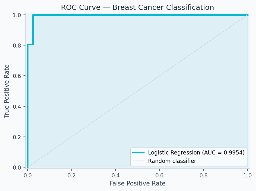
Code Implementation
train.pyimport numpy as np
from sklearn.datasets import load_breast_cancer
from sklearn.linear_model import LogisticRegression
from sklearn.model_selection import train_test_split
from sklearn.preprocessing import StandardScaler
from sklearn.metrics import roc_auc_score, classification_report
import joblib, os
def train(C=1.0, max_iter=1000, test_size=0.2, random_state=42):
data = load_breast_cancer()
X, y = data.data, data.target
X_train, X_test, y_train, y_test = train_test_split(
X, y, test_size=test_size, random_state=random_state, stratify=y
)
scaler = StandardScaler()
X_train_s = scaler.fit_transform(X_train)
X_test_s = scaler.transform(X_test)
model = LogisticRegression(C=C, max_iter=max_iter, solver='lbfgs')
model.fit(X_train_s, y_train)
y_pred = model.predict(X_test_s)
y_prob = model.predict_proba(X_test_s)[:, 1]
auc = roc_auc_score(y_test, y_prob)
print(f"AUC-ROC: {auc:.4f}")
print(classification_report(y_test, y_pred))
os.makedirs("artifacts", exist_ok=True)
joblib.dump(model, "artifacts/model.pkl")
joblib.dump(scaler, "artifacts/scaler.pkl")
return {"auc": auc, "model": model, "scaler": scaler}
if __name__ == "__main__":
train()Analysis & Evaluation
Where Your Intuition Breaks
High AUC means the model is well-calibrated. AUC measures ranking ability — whether positive examples score higher than negatives — not whether the predicted probabilities are accurate. A model with AUC 0.99 can be completely miscalibrated: predicting 0.9 for everything that's actually 0.7 base rate. Calibration (assessed with a reliability diagram or Brier score) is a separate property from discrimination. In medical and financial applications, both matter independently.
Metric Interpretation
| Metric | Result | Interpretation |
|---|---|---|
| Accuracy | 97.4% | High — but data is relatively clean |
| Area Under the Receiver Operating Characteristic Curve (AUC-ROC) | 0.9972 | Near-perfect discrimination |
| Recall (malignant) | 99% | Critical: missing cancer is expensive |
| Precision (benign) | 97% | Few false alarms |
For medical diagnosis, recall on the positive class (malignant = 0) is the critical metric — a false negative (missed cancer) costs far more than a false positive.
When Logistic Regression Fails
- Non-linear boundaries — XOR problem, circular decision boundaries
- Feature interactions — misses terms unless explicitly engineered
- Heavy class imbalance — use
class_weight='balanced'or Synthetic Minority Over-sampling Technique (SMOTE)
Regularization Effect
| C value | Effect | Use when |
|---|---|---|
| 0.01 | Heavy L2 — weights shrink toward 0 | Many irrelevant features |
| 1.0 | Balanced (default) | Good starting point |
| 100 | Near-unregularized | Features already curated |
Production-Ready Code
serve_api/app.pyfrom fastapi import FastAPI, HTTPException
from pydantic import BaseModel
import numpy as np
import joblib, os
app = FastAPI(title="Logistic Regression API")
model = joblib.load(os.environ.get("MODEL_PATH", "artifacts/model.pkl"))
scaler = joblib.load(os.environ.get("SCALER_PATH", "artifacts/scaler.pkl"))
class PredictRequest(BaseModel):
features: list[float]
class PredictResponse(BaseModel):
prediction: int
probability: float
label: str
@app.post("/predict", response_model=PredictResponse)
def predict(req: PredictRequest):
if len(req.features) != 30:
raise HTTPException(400, f"Expected 30 features, got {len(req.features)}")
x = np.array(req.features).reshape(1, -1)
x_scaled = scaler.transform(x)
pred = int(model.predict(x_scaled)[0])
prob = float(model.predict_proba(x_scaled)[0][1])
return PredictResponse(
prediction=pred,
probability=prob,
label="malignant" if pred == 0 else "benign",
)
@app.get("/health")
def health():
return {"status": "ok"}Before deploying: (1) validate input schema with Pydantic, (2) add /health for load balancer probes, (3) load model at startup not per-request, (4) version artifacts alongside model code, (5) log predictions with timestamps for drift monitoring.
Enjoying these notes?
Get new lessons delivered to your inbox. No spam.