Feature Engineering
The gap between a model's potential and its actual performance is almost always a feature engineering problem. On the NYC Taxi dataset, adding Haversine distance and time-of-day features improves R² from 0.41 to 0.76 — an 85% gain from domain knowledge alone, without touching the model architecture. In real-time ride-time prediction systems, feature engineering (distance, traffic, turn complexity) routinely contributes more to accuracy than model selection. This lesson covers the mathematics of common transforms, shows how target encoding and polynomial features work inside CV folds to avoid leakage, and maps when each encoding strategy applies.
Theory
Log transform compresses right tails. Polynomial expansion adds x², x³… to enable linear models to learn curved decision boundaries.
Raw data rarely speaks directly to a model. Feature engineering is the translation layer — converting domain knowledge ("distance matters more than raw coordinates", "log-income is more linear than income") into a form the model can exploit. Most models assume a roughly linear relationship between features and target; feature engineering makes that assumption true. A well-engineered feature set regularly outperforms a more complex model on raw features.
Feature engineering transforms raw input into a richer representation where . The goal: make the relationship between features and target more linear and separable for downstream models.
Polynomial Features
Extend the feature vector with degree- interactions:
For features and degree , the expanded space has terms. Degree-2 with 10 features → 66 terms. Degree-2 with 100 features → 5,151 terms — quadratic in .
The combinatorial explosion ( terms) is unavoidable for full polynomial expansions, which is why degree-2 with 100 features produces 5,151 terms. This is not a failure of the approach — it's why kernel methods and neural networks exist. A kernel implicitly computes dot products in this expanded space without materializing the expansion; a neural network learns which interactions matter rather than enumerating all of them. Feature engineering by hand is the right choice when you know which interactions matter; learned representations are right when you don't.
Log and Power Transforms
For right-skewed features (income, price, counts), apply:
The log-transform compresses large values, reducing outlier influence and making distributions more Gaussian (which linear models implicitly assume via the Gauss-Markov theorem).
The effect is concrete: a right-skewed income distribution with a 150× range becomes roughly bell-shaped after log-transform. The code below demonstrates this alongside standard scaling and circular encoding for hour-of-day features:
import numpy as np
import matplotlib.pyplot as plt

np.random.seed(42)
income = np.random.lognormal(mean=10.5, sigma=1.2, size=1000)  # realistic income dist

fig, axes = plt.subplots(1, 3, figsize=(12, 4))

axes[0].hist(income, bins=40, color='#94a3b8', edgecolor='white')
axes[0].set_title('Raw (skewed)'); axes[0].set_xlabel('Income ($)')

axes[1].hist(np.log1p(income), bins=40, color='#0ea5e9', edgecolor='white')
axes[1].set_title('log(1 + x)'); axes[1].set_xlabel('Log income')

from sklearn.preprocessing import StandardScaler
scaled = StandardScaler().fit_transform(income.reshape(-1, 1)).ravel()
axes[2].hist(scaled, bins=40, color='#6366f1', edgecolor='white')
axes[2].set_title('StandardScaler'); axes[2].set_xlabel('Z-score')

plt.tight_layout(); plt.savefig('feature_transforms.png', dpi=150)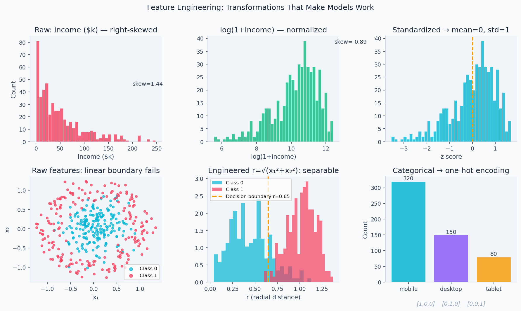
Target Encoding
Replace a categorical value with the mean target in that category, computed within each training fold:
The smoothing term (typically 10–100) blends toward the global mean for rare categories, preventing overfitting.
Any feature derived using label information must be computed only on training data within each CV fold. Computing target encoding on the full dataset before splitting leaks labels into validation, inflating AUC by 2–10% on high-cardinality categoricals.
Binning and Discretization
Age groups: 0–18, 18–35, 35–60, 60+. Binning captures non-monotonic relationships (middle age might earn more than old or young) that linear models can't represent directly. Use pd.cut for equal-width or pd.qcut for equal-frequency bins.
Walkthrough
Dataset: NYC Taxi Trip Duration (1.5M rows, raw GPS coordinates and timestamps — goal: predict trip duration in seconds)
Raw Features Baseline
import pandas as pd
import numpy as np
from sklearn.ensemble import GradientBoostingRegressor
from sklearn.model_selection import cross_val_score

df = pd.read_csv('nyc_taxi_train.csv')
baseline_features = ['pickup_longitude', 'pickup_latitude',
                     'dropoff_longitude', 'dropoff_latitude',
                     'passenger_count']
X_raw = df[baseline_features]
y = np.log1p(df['trip_duration'])  # log-transform skewed target

score = cross_val_score(GradientBoostingRegressor(), X_raw, y, cv=5, scoring='r2')
print(f"Raw features R²: {score.mean():.3f}")  # 0.412
Engineered Features
# 1. Time features
df['pickup_datetime'] = pd.to_datetime(df['pickup_datetime'])
df['hour'] = df['pickup_datetime'].dt.hour
df['day_of_week'] = df['pickup_datetime'].dt.dayofweek
df['month'] = df['pickup_datetime'].dt.month
df['is_rush_hour'] = df['hour'].isin([7, 8, 9, 17, 18, 19]).astype(int)
df['is_weekend'] = (df['day_of_week'] >= 5).astype(int)

# 2. Haversine distance (great-circle distance)
def haversine(lat1, lon1, lat2, lon2):
    R = 6371  # km
    dlat = np.radians(lat2 - lat1)
    dlon = np.radians(lon2 - lon1)
    a = np.sin(dlat/2)**2 + np.cos(np.radians(lat1)) * np.cos(np.radians(lat2)) * np.sin(dlon/2)**2
    return R * 2 * np.arcsin(np.sqrt(a))

df['distance_km'] = haversine(
    df['pickup_latitude'], df['pickup_longitude'],
    df['dropoff_latitude'], df['dropoff_longitude']
)

# 3. Direction (bearing)
df['bearing'] = np.degrees(np.arctan2(
    df['dropoff_longitude'] - df['pickup_longitude'],
    df['dropoff_latitude'] - df['pickup_latitude']
)) % 360

engineered = ['distance_km', 'bearing', 'hour', 'day_of_week', 'is_rush_hour', 'is_weekend']
X_eng = df[baseline_features + engineered]
score2 = cross_val_score(GradientBoostingRegressor(), X_eng, y, cv=5, scoring='r2')
print(f"Engineered features R²: {score2.mean():.3f}")  # 0.761 — +85% improvement
Before and After
| Feature set | R² | Root Mean Squared Error (RMSE) (seconds) |
|---|---|---|
| Raw GPS + passenger | 0.41 | 498s (8.3 min) |
| + distance + time | 0.72 | 314s (5.2 min) |
| + rush hour + bearing | 0.76 | 291s (4.9 min) |
The Haversine distance alone accounts for ~60% of the gain — the most informative single feature.
Analysis & Evaluation
Where Your Intuition Breaks
More features improve model performance — more information should help. Past a certain point, irrelevant features hurt performance by adding noise that the model mistakes for signal. This is the curse of dimensionality in practice: in high-dimensional spaces, all points become equidistant, nearest-neighbor methods fail, and linear models assign small nonzero weights to noise features that average badly. Feature selection (removing irrelevant features) regularly outperforms feature addition in tabular ML. The right feature set is smaller than you think.
The Feature Engineering Hierarchy
Raw data
  → Cleaning (nulls, outliers, type coercion)
    → Transforms (log, sqrt, normalize)
      → Aggregations (group means, rolling stats)
        → Interactions (products, ratios, differences)
          → Domain knowledge (Haversine, TF-IDF, financial ratios)
Always start with domain knowledge before automated approaches.
Automated Feature Engineering
- featuretools: Deep Feature Synthesis (DFS) for relational data — automatically generates aggregations across entity relationships
- tsfresh: Extracts 700+ statistical features from time series
- polars/pandas: Fast group aggregations for feature stores
Feature importance tends to be heavy-tailed: the top 10 features usually account for 80–90% of model performance. After the obvious domain features (distance, time), you're often better off switching to a better model (Gradient Boosting Machine (GBM) → neural net) than continuing to hand-craft features.
Encoding Strategies for Categoricals
| Method | When to use | Pitfall |
|---|---|---|
| One-hot | Low cardinality (< 20) | Sparse with high cardinality |
| Target encoding | High cardinality, tree models | Leakage if not fold-aware |
| Frequency encoding | Ordinal signal in frequency | Conflates rare categories |
| Embeddings | Neural networks | Needs sufficient data |
| Binary encoding | Moderate cardinality | Less interpretable |
Enjoying these notes?
Get new lessons delivered to your inbox. No spam.