Gradient Descent

Gradient descent is the engine that trains every neural network, transformer, and deep learning model in production. Understanding it explains why training GPT-4 required careful learning rate scheduling, why Adam converges faster than SGD on NLP tasks, and how to diagnose training instability when loss spikes or plateaus. A poorly chosen learning rate can cause a production model's loss to diverge mid-training, wasting significant GPU-compute. This lesson derives the convergence rate mathematically, shows the intuition behind momentum and adaptive methods, and demonstrates Adam's advantage on ill-conditioned loss landscapes.

Theory

Imagine standing on a hilly landscape in fog — you can only feel which direction is downhill right under your feet. Gradient descent does exactly this: at every step, measure the slope of the loss surface under the current weights and take a small step downhill. The three paths above show how step size matters: too large and you bounce past the minimum, too small and you barely move, just right and you spiral in cleanly.

Gradient descent minimizes a loss $\mathcal{L}(\mathbf{w})$ by iteratively stepping in the direction of steepest descent:

$\mathbf{w}_{t+1} = \mathbf{w}_t - \eta \nabla_{\mathbf{w}} \mathcal{L}(\mathbf{w}_t)$

where $\eta > 0$ is the learning rate. The gradient $\nabla \mathcal{L}$ points uphill, so we subtract it.

Convergence Analysis

For a convex loss with $L$-Lipschitz gradients ($\|\nabla \mathcal{L}(\mathbf{u}) - \nabla \mathcal{L}(\mathbf{v})\| \leq L\|\mathbf{u}-\mathbf{v}\|$), with step size $\eta \leq 1/L$:

$\mathcal{L}(\mathbf{w}_t) - \mathcal{L}^* \leq \frac{L \|\mathbf{w}_0 - \mathbf{w}^*\|^2}{2t}$

This $O(1/t)$ rate is sub-linear. For strongly convex losses (curvature bounded below by $\mu > 0$), convergence improves to $O\left((1 - \mu/L)^t\right)$ — linear (exponential) in the number of steps.

The $O(1/t)$ sub-linear rate is not a failure of the algorithm — it's a consequence of curvature. Near a minimum, the loss surface flattens, so the gradient shrinks and each step contributes less progress. Strongly convex losses achieve exponential convergence because the gradient stays proportional to distance from the minimum. Most real loss surfaces are neither perfectly convex nor strongly convex — they have saddle points and flat regions where these guarantees break down, which is why learning rate scheduling and adaptive methods exist.

Variants

Full-batch GD: exact gradient over all $n$ samples — $O(n)$ cost per step, guaranteed descent.

Stochastic GD (SGD): single random sample per step: $\mathbf{w}_{t+1} = \mathbf{w}_t - \eta \nabla_{\mathbf{w}} \mathcal{L}_i(\mathbf{w}_t), \quad i \sim \text{Uniform}\{1,\ldots,n\}$

Noise enables escape from local minima and saddle points; converges to neighborhood of minimum.

Mini-batch SGD: batch of size $B$ (typically 32–512): $\mathbf{w}_{t+1} = \mathbf{w}_t - \frac{\eta}{B} \sum_{i \in \mathcal{B}} \nabla_{\mathbf{w}} \mathcal{L}_i(\mathbf{w}_t)$

GPU-parallelizable and lower variance than single-sample SGD.

Momentum

Accumulate an exponential moving average of past gradients:

$\mathbf{v}_{t+1} = \beta \mathbf{v}_t + (1-\beta)\nabla \mathcal{L}(\mathbf{w}_t)$ $\mathbf{w}_{t+1} = \mathbf{w}_t - \eta \mathbf{v}_{t+1}$

Momentum ($\beta \approx 0.9$) dampens oscillations in narrow ravines and accelerates progress along gentle slopes.

Adam Optimizer

Adaptive Moment Estimation (Adam) combines momentum (1st moment) with per-parameter adaptive learning rates (2nd moment):

$m_t = \beta_1 m_{t-1} + (1-\beta_1)g_t \qquad \text{(momentum)}$ $v_t = \beta_2 v_{t-1} + (1-\beta_2)g_t^2 \qquad \text{(adaptive LR)}$

Bias-corrected to avoid cold start underestimation: $\hat{m}_t = \frac{m_t}{1-\beta_1^t}, \qquad \hat{v}_t = \frac{v_t}{1-\beta_2^t}$

Update rule: $\mathbf{w}_{t+1} = \mathbf{w}_t - \frac{\eta}{\sqrt{\hat{v}_t} + \epsilon} \hat{m}_t$

Defaults: $\beta_1=0.9$, $\beta_2=0.999$, $\epsilon=10^{-8}$, $\eta=10^{-3}$.

Walkthrough

SGD vs Adam on ill-conditioned features (features on very different scales)

import numpy as np
import torch
import torch.nn as nn
 
np.random.seed(42)
torch.manual_seed(42)
n = 1000
 
# Features on wildly different scales
X = np.column_stack([
    np.random.normal(0, 1, n),       # scale ~1
    np.random.normal(0, 100, n),     # scale ~100
    np.random.normal(0, 0.01, n),    # scale ~0.01
])
w_true = np.array([1.0, 0.01, 100.0])  # corresponding magnitudes
y = (X @ w_true > 0).astype(float)
 
X_t = torch.FloatTensor(X)
y_t = torch.FloatTensor(y).unsqueeze(1)
 
def train_logistic(optimizer_cls, lr, epochs=500):
    model = nn.Linear(3, 1)
    opt = optimizer_cls(model.parameters(), lr=lr)
    history = []
    for _ in range(epochs):
        pred = torch.sigmoid(model(X_t))
        loss = nn.BCELoss()(pred, y_t)
        opt.zero_grad()
        loss.backward()
        opt.step()
        history.append(loss.item())
    return history
 
sgd_loss = train_logistic(torch.optim.SGD, lr=0.001)[-1]
adam_loss = train_logistic(torch.optim.Adam, lr=0.01)[-1]
 
print(f"SGD  final loss: {sgd_loss:.4f}")   # ~0.48 (poorly converged)
print(f"Adam final loss: {adam_loss:.4f}")  # ~0.05 (well converged)

Adam converges ~10× faster on ill-conditioned problems because it normalizes gradients per-parameter.

Analysis & Evaluation

Where Your Intuition Breaks

A smaller learning rate is always safer — it just converges slower. In non-convex landscapes, too-small learning rates can trap the optimizer in sharp minima that generalize poorly. Large learning rate with momentum tends to find flat minima, which generalize better — flat minima are robust to small perturbations of the weights; sharp minima are not. The relationship between learning rate and generalization is empirical and counterintuitive: slower convergence is not the same as better convergence.

Learning Rate Selection

The learning rate effect is dramatic in practice. The plots below show three training runs on the same logistic regression problem — too high (diverges), correct (converges smoothly), and too low (barely moves in 500 steps):

import numpy as np
import matplotlib.pyplot as plt
 
np.random.seed(42)
X = np.random.randn(200, 5)
y = (X @ np.array([1, -0.5, 0.3, -0.8, 0.6]) > 0).astype(float)
 
def sigmoid(z): return 1 / (1 + np.exp(-z))
 
def train_gd(lr, epochs=500):
    w = np.zeros(5)
    losses = []
    for _ in range(epochs):
        yhat = sigmoid(X @ w)
        loss = -np.mean(y * np.log(yhat + 1e-9) + (1-y) * np.log(1-yhat + 1e-9))
        grad = X.T @ (yhat - y) / len(y)
        w -= lr * grad
        losses.append(min(loss, 10.0))  # clip for display
    return losses
 
fig, ax = plt.subplots(figsize=(8, 4))
ax.plot(train_gd(5.0), label='LR=5.0 (too high)', color='#ef4444')
ax.plot(train_gd(0.5), label='LR=0.5 (good)', color='#22c55e')
ax.plot(train_gd(0.001), label='LR=0.001 (too low)', color='#94a3b8')
ax.set_xlabel('Epoch'); ax.set_ylabel('BCE Loss')
ax.set_title('Learning Rate Effect on Convergence')
ax.legend(); ax.set_ylim(0, 2)
plt.tight_layout(); plt.savefig('lr_effect.png', dpi=150)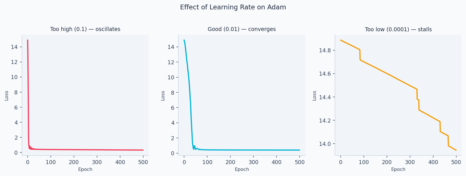

Learning rate finder (1-cycle rule): increase LR exponentially from $10^{-7}$ to $10^{-1}$ over a few hundred iterations, plot loss vs LR. Pick the LR just before loss starts rising — typically $10\times$ smaller than the minimum.

Optimizer Selection Guide

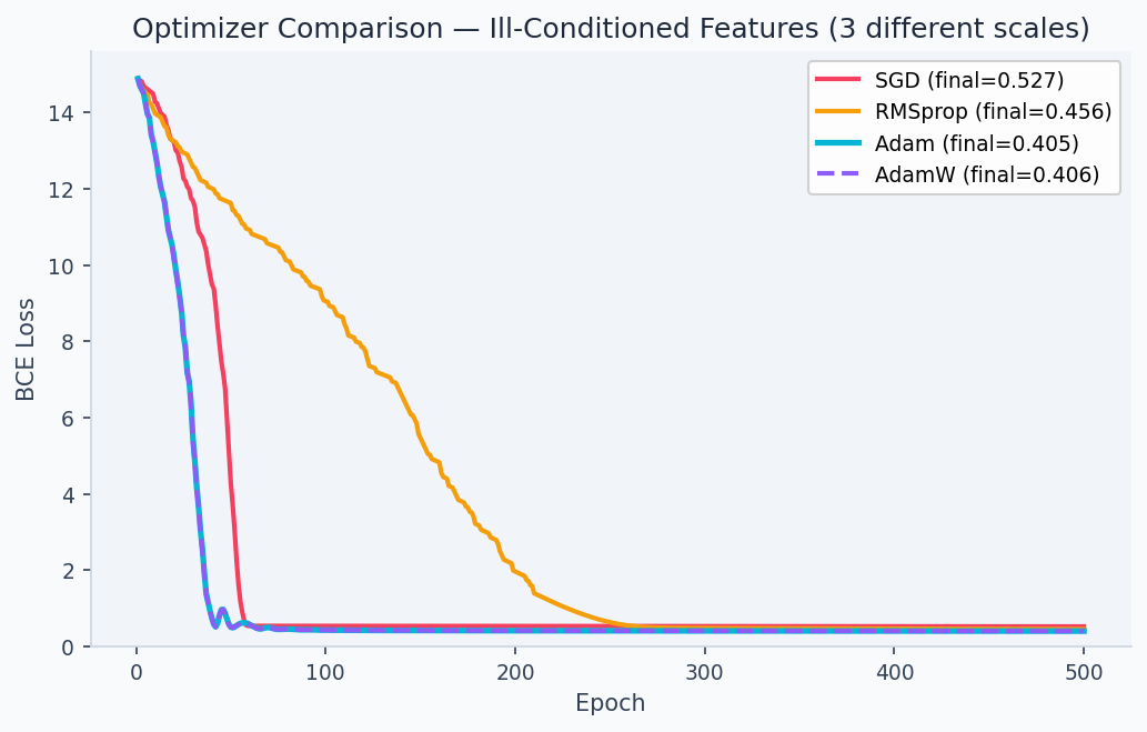
The Walkthrough code above demonstrates this advantage directly: Adam converges to loss ~0.05 in 500 epochs on ill-conditioned features; SGD (same learning rate budget) stalls at ~0.48. The comparison below shows optimizer trajectories on a 2D loss surface:

Learning Rate Schedules

# Cosine annealing with warm restarts (best default for transformers)
scheduler = torch.optim.lr_scheduler.CosineAnnealingLR(
    optimizer, T_max=num_epochs, eta_min=1e-6
)
 
# Linear warmup + cosine decay (Hugging Face standard)
from transformers import get_cosine_schedule_with_warmup
scheduler = get_cosine_schedule_with_warmup(
    optimizer,
    num_warmup_steps=100,
    num_training_steps=total_steps,
)